Updated license

Branches diverged because of work on the readme and code separately. Now they will be put back together.

.gitignore

@@ -105,5 +105,5 @@ dmypy.json
 .pyre/
 
 # Exclude SPIE/Data en SPIE/Figures folders
-scripts/SPIE/data
+# scripts/SPIE/data
-scripts/SPIE/figures
+# scripts/SPIE/figures

LICENSE.txt

@@ -0,0 +1,674 @@
+                    GNU GENERAL PUBLIC LICENSE
+                       Version 3, 29 June 2007
+
+ Copyright (C) 2007 Free Software Foundation, Inc. <https://fsf.org/>
+ Everyone is permitted to copy and distribute verbatim copies
+ of this license document, but changing it is not allowed.
+
+                            Preamble
+
+  The GNU General Public License is a free, copyleft license for
+software and other kinds of works.
+
+  The licenses for most software and other practical works are designed
+to take away your freedom to share and change the works.  By contrast,
+the GNU General Public License is intended to guarantee your freedom to
+share and change all versions of a program--to make sure it remains free
+software for all its users.  We, the Free Software Foundation, use the
+GNU General Public License for most of our software; it applies also to
+any other work released this way by its authors.  You can apply it to
+your programs, too.
+
+  When we speak of free software, we are referring to freedom, not
+price.  Our General Public Licenses are designed to make sure that you
+have the freedom to distribute copies of free software (and charge for
+them if you wish), that you receive source code or can get it if you
+want it, that you can change the software or use pieces of it in new
+free programs, and that you know you can do these things.
+
+  To protect your rights, we need to prevent others from denying you
+these rights or asking you to surrender the rights.  Therefore, you have
+certain responsibilities if you distribute copies of the software, or if
+you modify it: responsibilities to respect the freedom of others.
+
+  For example, if you distribute copies of such a program, whether
+gratis or for a fee, you must pass on to the recipients the same
+freedoms that you received.  You must make sure that they, too, receive
+or can get the source code.  And you must show them these terms so they
+know their rights.
+
+  Developers that use the GNU GPL protect your rights with two steps:
+(1) assert copyright on the software, and (2) offer you this License
+giving you legal permission to copy, distribute and/or modify it.
+
+  For the developers' and authors' protection, the GPL clearly explains
+that there is no warranty for this free software.  For both users' and
+authors' sake, the GPL requires that modified versions be marked as
+changed, so that their problems will not be attributed erroneously to
+authors of previous versions.
+
+  Some devices are designed to deny users access to install or run
+modified versions of the software inside them, although the manufacturer
+can do so.  This is fundamentally incompatible with the aim of
+protecting users' freedom to change the software.  The systematic
+pattern of such abuse occurs in the area of products for individuals to
+use, which is precisely where it is most unacceptable.  Therefore, we
+have designed this version of the GPL to prohibit the practice for those
+products.  If such problems arise substantially in other domains, we
+stand ready to extend this provision to those domains in future versions
+of the GPL, as needed to protect the freedom of users.
+
+  Finally, every program is threatened constantly by software patents.
+States should not allow patents to restrict development and use of
+software on general-purpose computers, but in those that do, we wish to
+avoid the special danger that patents applied to a free program could
+make it effectively proprietary.  To prevent this, the GPL assures that
+patents cannot be used to render the program non-free.
+
+  The precise terms and conditions for copying, distribution and
+modification follow.
+
+                       TERMS AND CONDITIONS
+
+  0. Definitions.
+
+  "This License" refers to version 3 of the GNU General Public License.
+
+  "Copyright" also means copyright-like laws that apply to other kinds of
+works, such as semiconductor masks.
+
+  "The Program" refers to any copyrightable work licensed under this
+License.  Each licensee is addressed as "you".  "Licensees" and
+"recipients" may be individuals or organizations.
+
+  To "modify" a work means to copy from or adapt all or part of the work
+in a fashion requiring copyright permission, other than the making of an
+exact copy.  The resulting work is called a "modified version" of the
+earlier work or a work "based on" the earlier work.
+
+  A "covered work" means either the unmodified Program or a work based
+on the Program.
+
+  To "propagate" a work means to do anything with it that, without
+permission, would make you directly or secondarily liable for
+infringement under applicable copyright law, except executing it on a
+computer or modifying a private copy.  Propagation includes copying,
+distribution (with or without modification), making available to the
+public, and in some countries other activities as well.
+
+  To "convey" a work means any kind of propagation that enables other
+parties to make or receive copies.  Mere interaction with a user through
+a computer network, with no transfer of a copy, is not conveying.
+
+  An interactive user interface displays "Appropriate Legal Notices"
+to the extent that it includes a convenient and prominently visible
+feature that (1) displays an appropriate copyright notice, and (2)
+tells the user that there is no warranty for the work (except to the
+extent that warranties are provided), that licensees may convey the
+work under this License, and how to view a copy of this License.  If
+the interface presents a list of user commands or options, such as a
+menu, a prominent item in the list meets this criterion.
+
+  1. Source Code.
+
+  The "source code" for a work means the preferred form of the work
+for making modifications to it.  "Object code" means any non-source
+form of a work.
+
+  A "Standard Interface" means an interface that either is an official
+standard defined by a recognized standards body, or, in the case of
+interfaces specified for a particular programming language, one that
+is widely used among developers working in that language.
+
+  The "System Libraries" of an executable work include anything, other
+than the work as a whole, that (a) is included in the normal form of
+packaging a Major Component, but which is not part of that Major
+Component, and (b) serves only to enable use of the work with that
+Major Component, or to implement a Standard Interface for which an
+implementation is available to the public in source code form.  A
+"Major Component", in this context, means a major essential component
+(kernel, window system, and so on) of the specific operating system
+(if any) on which the executable work runs, or a compiler used to
+produce the work, or an object code interpreter used to run it.
+
+  The "Corresponding Source" for a work in object code form means all
+the source code needed to generate, install, and (for an executable
+work) run the object code and to modify the work, including scripts to
+control those activities.  However, it does not include the work's
+System Libraries, or general-purpose tools or generally available free
+programs which are used unmodified in performing those activities but
+which are not part of the work.  For example, Corresponding Source
+includes interface definition files associated with source files for
+the work, and the source code for shared libraries and dynamically
+linked subprograms that the work is specifically designed to require,
+such as by intimate data communication or control flow between those
+subprograms and other parts of the work.
+
+  The Corresponding Source need not include anything that users
+can regenerate automatically from other parts of the Corresponding
+Source.
+
+  The Corresponding Source for a work in source code form is that
+same work.
+
+  2. Basic Permissions.
+
+  All rights granted under this License are granted for the term of
+copyright on the Program, and are irrevocable provided the stated
+conditions are met.  This License explicitly affirms your unlimited
+permission to run the unmodified Program.  The output from running a
+covered work is covered by this License only if the output, given its
+content, constitutes a covered work.  This License acknowledges your
+rights of fair use or other equivalent, as provided by copyright law.
+
+  You may make, run and propagate covered works that you do not
+convey, without conditions so long as your license otherwise remains
+in force.  You may convey covered works to others for the sole purpose
+of having them make modifications exclusively for you, or provide you
+with facilities for running those works, provided that you comply with
+the terms of this License in conveying all material for which you do
+not control copyright.  Those thus making or running the covered works
+for you must do so exclusively on your behalf, under your direction
+and control, on terms that prohibit them from making any copies of
+your copyrighted material outside their relationship with you.
+
+  Conveying under any other circumstances is permitted solely under
+the conditions stated below.  Sublicensing is not allowed; section 10
+makes it unnecessary.
+
+  3. Protecting Users' Legal Rights From Anti-Circumvention Law.
+
+  No covered work shall be deemed part of an effective technological
+measure under any applicable law fulfilling obligations under article
+11 of the WIPO copyright treaty adopted on 20 December 1996, or
+similar laws prohibiting or restricting circumvention of such
+measures.
+
+  When you convey a covered work, you waive any legal power to forbid
+circumvention of technological measures to the extent such circumvention
+is effected by exercising rights under this License with respect to
+the covered work, and you disclaim any intention to limit operation or
+modification of the work as a means of enforcing, against the work's
+users, your or third parties' legal rights to forbid circumvention of
+technological measures.
+
+  4. Conveying Verbatim Copies.
+
+  You may convey verbatim copies of the Program's source code as you
+receive it, in any medium, provided that you conspicuously and
+appropriately publish on each copy an appropriate copyright notice;
+keep intact all notices stating that this License and any
+non-permissive terms added in accord with section 7 apply to the code;
+keep intact all notices of the absence of any warranty; and give all
+recipients a copy of this License along with the Program.
+
+  You may charge any price or no price for each copy that you convey,
+and you may offer support or warranty protection for a fee.
+
+  5. Conveying Modified Source Versions.
+
+  You may convey a work based on the Program, or the modifications to
+produce it from the Program, in the form of source code under the
+terms of section 4, provided that you also meet all of these conditions:
+
+    a) The work must carry prominent notices stating that you modified
+    it, and giving a relevant date.
+
+    b) The work must carry prominent notices stating that it is
+    released under this License and any conditions added under section
+    7.  This requirement modifies the requirement in section 4 to
+    "keep intact all notices".
+
+    c) You must license the entire work, as a whole, under this
+    License to anyone who comes into possession of a copy.  This
+    License will therefore apply, along with any applicable section 7
+    additional terms, to the whole of the work, and all its parts,
+    regardless of how they are packaged.  This License gives no
+    permission to license the work in any other way, but it does not
+    invalidate such permission if you have separately received it.
+
+    d) If the work has interactive user interfaces, each must display
+    Appropriate Legal Notices; however, if the Program has interactive
+    interfaces that do not display Appropriate Legal Notices, your
+    work need not make them do so.
+
+  A compilation of a covered work with other separate and independent
+works, which are not by their nature extensions of the covered work,
+and which are not combined with it such as to form a larger program,
+in or on a volume of a storage or distribution medium, is called an
+"aggregate" if the compilation and its resulting copyright are not
+used to limit the access or legal rights of the compilation's users
+beyond what the individual works permit.  Inclusion of a covered work
+in an aggregate does not cause this License to apply to the other
+parts of the aggregate.
+
+  6. Conveying Non-Source Forms.
+
+  You may convey a covered work in object code form under the terms
+of sections 4 and 5, provided that you also convey the
+machine-readable Corresponding Source under the terms of this License,
+in one of these ways:
+
+    a) Convey the object code in, or embodied in, a physical product
+    (including a physical distribution medium), accompanied by the
+    Corresponding Source fixed on a durable physical medium
+    customarily used for software interchange.
+
+    b) Convey the object code in, or embodied in, a physical product
+    (including a physical distribution medium), accompanied by a
+    written offer, valid for at least three years and valid for as
+    long as you offer spare parts or customer support for that product
+    model, to give anyone who possesses the object code either (1) a
+    copy of the Corresponding Source for all the software in the
+    product that is covered by this License, on a durable physical
+    medium customarily used for software interchange, for a price no
+    more than your reasonable cost of physically performing this
+    conveying of source, or (2) access to copy the
+    Corresponding Source from a network server at no charge.
+
+    c) Convey individual copies of the object code with a copy of the
+    written offer to provide the Corresponding Source.  This
+    alternative is allowed only occasionally and noncommercially, and
+    only if you received the object code with such an offer, in accord
+    with subsection 6b.
+
+    d) Convey the object code by offering access from a designated
+    place (gratis or for a charge), and offer equivalent access to the
+    Corresponding Source in the same way through the same place at no
+    further charge.  You need not require recipients to copy the
+    Corresponding Source along with the object code.  If the place to
+    copy the object code is a network server, the Corresponding Source
+    may be on a different server (operated by you or a third party)
+    that supports equivalent copying facilities, provided you maintain
+    clear directions next to the object code saying where to find the
+    Corresponding Source.  Regardless of what server hosts the
+    Corresponding Source, you remain obligated to ensure that it is
+    available for as long as needed to satisfy these requirements.
+
+    e) Convey the object code using peer-to-peer transmission, provided
+    you inform other peers where the object code and Corresponding
+    Source of the work are being offered to the general public at no
+    charge under subsection 6d.
+
+  A separable portion of the object code, whose source code is excluded
+from the Corresponding Source as a System Library, need not be
+included in conveying the object code work.
+
+  A "User Product" is either (1) a "consumer product", which means any
+tangible personal property which is normally used for personal, family,
+or household purposes, or (2) anything designed or sold for incorporation
+into a dwelling.  In determining whether a product is a consumer product,
+doubtful cases shall be resolved in favor of coverage.  For a particular
+product received by a particular user, "normally used" refers to a
+typical or common use of that class of product, regardless of the status
+of the particular user or of the way in which the particular user
+actually uses, or expects or is expected to use, the product.  A product
+is a consumer product regardless of whether the product has substantial
+commercial, industrial or non-consumer uses, unless such uses represent
+the only significant mode of use of the product.
+
+  "Installation Information" for a User Product means any methods,
+procedures, authorization keys, or other information required to install
+and execute modified versions of a covered work in that User Product from
+a modified version of its Corresponding Source.  The information must
+suffice to ensure that the continued functioning of the modified object
+code is in no case prevented or interfered with solely because
+modification has been made.
+
+  If you convey an object code work under this section in, or with, or
+specifically for use in, a User Product, and the conveying occurs as
+part of a transaction in which the right of possession and use of the
+User Product is transferred to the recipient in perpetuity or for a
+fixed term (regardless of how the transaction is characterized), the
+Corresponding Source conveyed under this section must be accompanied
+by the Installation Information.  But this requirement does not apply
+if neither you nor any third party retains the ability to install
+modified object code on the User Product (for example, the work has
+been installed in ROM).
+
+  The requirement to provide Installation Information does not include a
+requirement to continue to provide support service, warranty, or updates
+for a work that has been modified or installed by the recipient, or for
+the User Product in which it has been modified or installed.  Access to a
+network may be denied when the modification itself materially and
+adversely affects the operation of the network or violates the rules and
+protocols for communication across the network.
+
+  Corresponding Source conveyed, and Installation Information provided,
+in accord with this section must be in a format that is publicly
+documented (and with an implementation available to the public in
+source code form), and must require no special password or key for
+unpacking, reading or copying.
+
+  7. Additional Terms.
+
+  "Additional permissions" are terms that supplement the terms of this
+License by making exceptions from one or more of its conditions.
+Additional permissions that are applicable to the entire Program shall
+be treated as though they were included in this License, to the extent
+that they are valid under applicable law.  If additional permissions
+apply only to part of the Program, that part may be used separately
+under those permissions, but the entire Program remains governed by
+this License without regard to the additional permissions.
+
+  When you convey a copy of a covered work, you may at your option
+remove any additional permissions from that copy, or from any part of
+it.  (Additional permissions may be written to require their own
+removal in certain cases when you modify the work.)  You may place
+additional permissions on material, added by you to a covered work,
+for which you have or can give appropriate copyright permission.
+
+  Notwithstanding any other provision of this License, for material you
+add to a covered work, you may (if authorized by the copyright holders of
+that material) supplement the terms of this License with terms:
+
+    a) Disclaiming warranty or limiting liability differently from the
+    terms of sections 15 and 16 of this License; or
+
+    b) Requiring preservation of specified reasonable legal notices or
+    author attributions in that material or in the Appropriate Legal
+    Notices displayed by works containing it; or
+
+    c) Prohibiting misrepresentation of the origin of that material, or
+    requiring that modified versions of such material be marked in
+    reasonable ways as different from the original version; or
+
+    d) Limiting the use for publicity purposes of names of licensors or
+    authors of the material; or
+
+    e) Declining to grant rights under trademark law for use of some
+    trade names, trademarks, or service marks; or
+
+    f) Requiring indemnification of licensors and authors of that
+    material by anyone who conveys the material (or modified versions of
+    it) with contractual assumptions of liability to the recipient, for
+    any liability that these contractual assumptions directly impose on
+    those licensors and authors.
+
+  All other non-permissive additional terms are considered "further
+restrictions" within the meaning of section 10.  If the Program as you
+received it, or any part of it, contains a notice stating that it is
+governed by this License along with a term that is a further
+restriction, you may remove that term.  If a license document contains
+a further restriction but permits relicensing or conveying under this
+License, you may add to a covered work material governed by the terms
+of that license document, provided that the further restriction does
+not survive such relicensing or conveying.
+
+  If you add terms to a covered work in accord with this section, you
+must place, in the relevant source files, a statement of the
+additional terms that apply to those files, or a notice indicating
+where to find the applicable terms.
+
+  Additional terms, permissive or non-permissive, may be stated in the
+form of a separately written license, or stated as exceptions;
+the above requirements apply either way.
+
+  8. Termination.
+
+  You may not propagate or modify a covered work except as expressly
+provided under this License.  Any attempt otherwise to propagate or
+modify it is void, and will automatically terminate your rights under
+this License (including any patent licenses granted under the third
+paragraph of section 11).
+
+  However, if you cease all violation of this License, then your
+license from a particular copyright holder is reinstated (a)
+provisionally, unless and until the copyright holder explicitly and
+finally terminates your license, and (b) permanently, if the copyright
+holder fails to notify you of the violation by some reasonable means
+prior to 60 days after the cessation.
+
+  Moreover, your license from a particular copyright holder is
+reinstated permanently if the copyright holder notifies you of the
+violation by some reasonable means, this is the first time you have
+received notice of violation of this License (for any work) from that
+copyright holder, and you cure the violation prior to 30 days after
+your receipt of the notice.
+
+  Termination of your rights under this section does not terminate the
+licenses of parties who have received copies or rights from you under
+this License.  If your rights have been terminated and not permanently
+reinstated, you do not qualify to receive new licenses for the same
+material under section 10.
+
+  9. Acceptance Not Required for Having Copies.
+
+  You are not required to accept this License in order to receive or
+run a copy of the Program.  Ancillary propagation of a covered work
+occurring solely as a consequence of using peer-to-peer transmission
+to receive a copy likewise does not require acceptance.  However,
+nothing other than this License grants you permission to propagate or
+modify any covered work.  These actions infringe copyright if you do
+not accept this License.  Therefore, by modifying or propagating a
+covered work, you indicate your acceptance of this License to do so.
+
+  10. Automatic Licensing of Downstream Recipients.
+
+  Each time you convey a covered work, the recipient automatically
+receives a license from the original licensors, to run, modify and
+propagate that work, subject to this License.  You are not responsible
+for enforcing compliance by third parties with this License.
+
+  An "entity transaction" is a transaction transferring control of an
+organization, or substantially all assets of one, or subdividing an
+organization, or merging organizations.  If propagation of a covered
+work results from an entity transaction, each party to that
+transaction who receives a copy of the work also receives whatever
+licenses to the work the party's predecessor in interest had or could
+give under the previous paragraph, plus a right to possession of the
+Corresponding Source of the work from the predecessor in interest, if
+the predecessor has it or can get it with reasonable efforts.
+
+  You may not impose any further restrictions on the exercise of the
+rights granted or affirmed under this License.  For example, you may
+not impose a license fee, royalty, or other charge for exercise of
+rights granted under this License, and you may not initiate litigation
+(including a cross-claim or counterclaim in a lawsuit) alleging that
+any patent claim is infringed by making, using, selling, offering for
+sale, or importing the Program or any portion of it.
+
+  11. Patents.
+
+  A "contributor" is a copyright holder who authorizes use under this
+License of the Program or a work on which the Program is based.  The
+work thus licensed is called the contributor's "contributor version".
+
+  A contributor's "essential patent claims" are all patent claims
+owned or controlled by the contributor, whether already acquired or
+hereafter acquired, that would be infringed by some manner, permitted
+by this License, of making, using, or selling its contributor version,
+but do not include claims that would be infringed only as a
+consequence of further modification of the contributor version.  For
+purposes of this definition, "control" includes the right to grant
+patent sublicenses in a manner consistent with the requirements of
+this License.
+
+  Each contributor grants you a non-exclusive, worldwide, royalty-free
+patent license under the contributor's essential patent claims, to
+make, use, sell, offer for sale, import and otherwise run, modify and
+propagate the contents of its contributor version.
+
+  In the following three paragraphs, a "patent license" is any express
+agreement or commitment, however denominated, not to enforce a patent
+(such as an express permission to practice a patent or covenant not to
+sue for patent infringement).  To "grant" such a patent license to a
+party means to make such an agreement or commitment not to enforce a
+patent against the party.
+
+  If you convey a covered work, knowingly relying on a patent license,
+and the Corresponding Source of the work is not available for anyone
+to copy, free of charge and under the terms of this License, through a
+publicly available network server or other readily accessible means,
+then you must either (1) cause the Corresponding Source to be so
+available, or (2) arrange to deprive yourself of the benefit of the
+patent license for this particular work, or (3) arrange, in a manner
+consistent with the requirements of this License, to extend the patent
+license to downstream recipients.  "Knowingly relying" means you have
+actual knowledge that, but for the patent license, your conveying the
+covered work in a country, or your recipient's use of the covered work
+in a country, would infringe one or more identifiable patents in that
+country that you have reason to believe are valid.
+
+  If, pursuant to or in connection with a single transaction or
+arrangement, you convey, or propagate by procuring conveyance of, a
+covered work, and grant a patent license to some of the parties
+receiving the covered work authorizing them to use, propagate, modify
+or convey a specific copy of the covered work, then the patent license
+you grant is automatically extended to all recipients of the covered
+work and works based on it.
+
+  A patent license is "discriminatory" if it does not include within
+the scope of its coverage, prohibits the exercise of, or is
+conditioned on the non-exercise of one or more of the rights that are
+specifically granted under this License.  You may not convey a covered
+work if you are a party to an arrangement with a third party that is
+in the business of distributing software, under which you make payment
+to the third party based on the extent of your activity of conveying
+the work, and under which the third party grants, to any of the
+parties who would receive the covered work from you, a discriminatory
+patent license (a) in connection with copies of the covered work
+conveyed by you (or copies made from those copies), or (b) primarily
+for and in connection with specific products or compilations that
+contain the covered work, unless you entered into that arrangement,
+or that patent license was granted, prior to 28 March 2007.
+
+  Nothing in this License shall be construed as excluding or limiting
+any implied license or other defenses to infringement that may
+otherwise be available to you under applicable patent law.
+
+  12. No Surrender of Others' Freedom.
+
+  If conditions are imposed on you (whether by court order, agreement or
+otherwise) that contradict the conditions of this License, they do not
+excuse you from the conditions of this License.  If you cannot convey a
+covered work so as to satisfy simultaneously your obligations under this
+License and any other pertinent obligations, then as a consequence you may
+not convey it at all.  For example, if you agree to terms that obligate you
+to collect a royalty for further conveying from those to whom you convey
+the Program, the only way you could satisfy both those terms and this
+License would be to refrain entirely from conveying the Program.
+
+  13. Use with the GNU Affero General Public License.
+
+  Notwithstanding any other provision of this License, you have
+permission to link or combine any covered work with a work licensed
+under version 3 of the GNU Affero General Public License into a single
+combined work, and to convey the resulting work.  The terms of this
+License will continue to apply to the part which is the covered work,
+but the special requirements of the GNU Affero General Public License,
+section 13, concerning interaction through a network will apply to the
+combination as such.
+
+  14. Revised Versions of this License.
+
+  The Free Software Foundation may publish revised and/or new versions of
+the GNU General Public License from time to time.  Such new versions will
+be similar in spirit to the present version, but may differ in detail to
+address new problems or concerns.
+
+  Each version is given a distinguishing version number.  If the
+Program specifies that a certain numbered version of the GNU General
+Public License "or any later version" applies to it, you have the
+option of following the terms and conditions either of that numbered
+version or of any later version published by the Free Software
+Foundation.  If the Program does not specify a version number of the
+GNU General Public License, you may choose any version ever published
+by the Free Software Foundation.
+
+  If the Program specifies that a proxy can decide which future
+versions of the GNU General Public License can be used, that proxy's
+public statement of acceptance of a version permanently authorizes you
+to choose that version for the Program.
+
+  Later license versions may give you additional or different
+permissions.  However, no additional obligations are imposed on any
+author or copyright holder as a result of your choosing to follow a
+later version.
+
+  15. Disclaimer of Warranty.
+
+  THERE IS NO WARRANTY FOR THE PROGRAM, TO THE EXTENT PERMITTED BY
+APPLICABLE LAW.  EXCEPT WHEN OTHERWISE STATED IN WRITING THE COPYRIGHT
+HOLDERS AND/OR OTHER PARTIES PROVIDE THE PROGRAM "AS IS" WITHOUT WARRANTY
+OF ANY KIND, EITHER EXPRESSED OR IMPLIED, INCLUDING, BUT NOT LIMITED TO,
+THE IMPLIED WARRANTIES OF MERCHANTABILITY AND FITNESS FOR A PARTICULAR
+PURPOSE.  THE ENTIRE RISK AS TO THE QUALITY AND PERFORMANCE OF THE PROGRAM
+IS WITH YOU.  SHOULD THE PROGRAM PROVE DEFECTIVE, YOU ASSUME THE COST OF
+ALL NECESSARY SERVICING, REPAIR OR CORRECTION.
+
+  16. Limitation of Liability.
+
+  IN NO EVENT UNLESS REQUIRED BY APPLICABLE LAW OR AGREED TO IN WRITING
+WILL ANY COPYRIGHT HOLDER, OR ANY OTHER PARTY WHO MODIFIES AND/OR CONVEYS
+THE PROGRAM AS PERMITTED ABOVE, BE LIABLE TO YOU FOR DAMAGES, INCLUDING ANY
+GENERAL, SPECIAL, INCIDENTAL OR CONSEQUENTIAL DAMAGES ARISING OUT OF THE
+USE OR INABILITY TO USE THE PROGRAM (INCLUDING BUT NOT LIMITED TO LOSS OF
+DATA OR DATA BEING RENDERED INACCURATE OR LOSSES SUSTAINED BY YOU OR THIRD
+PARTIES OR A FAILURE OF THE PROGRAM TO OPERATE WITH ANY OTHER PROGRAMS),
+EVEN IF SUCH HOLDER OR OTHER PARTY HAS BEEN ADVISED OF THE POSSIBILITY OF
+SUCH DAMAGES.
+
+  17. Interpretation of Sections 15 and 16.
+
+  If the disclaimer of warranty and limitation of liability provided
+above cannot be given local legal effect according to their terms,
+reviewing courts shall apply local law that most closely approximates
+an absolute waiver of all civil liability in connection with the
+Program, unless a warranty or assumption of liability accompanies a
+copy of the Program in return for a fee.
+
+                     END OF TERMS AND CONDITIONS
+
+            How to Apply These Terms to Your New Programs
+
+  If you develop a new program, and you want it to be of the greatest
+possible use to the public, the best way to achieve this is to make it
+free software which everyone can redistribute and change under these terms.
+
+  To do so, attach the following notices to the program.  It is safest
+to attach them to the start of each source file to most effectively
+state the exclusion of warranty; and each file should have at least
+the "copyright" line and a pointer to where the full notice is found.
+
+    <one line to give the program's name and a brief idea of what it does.>
+    Copyright (C) <year>  <name of author>
+
+    This program is free software: you can redistribute it and/or modify
+    it under the terms of the GNU General Public License as published by
+    the Free Software Foundation, either version 3 of the License, or
+    (at your option) any later version.
+
+    This program is distributed in the hope that it will be useful,
+    but WITHOUT ANY WARRANTY; without even the implied warranty of
+    MERCHANTABILITY or FITNESS FOR A PARTICULAR PURPOSE.  See the
+    GNU General Public License for more details.
+
+    You should have received a copy of the GNU General Public License
+    along with this program.  If not, see <https://www.gnu.org/licenses/>.
+
+Also add information on how to contact you by electronic and paper mail.
+
+  If the program does terminal interaction, make it output a short
+notice like this when it starts in an interactive mode:
+
+    <program>  Copyright (C) <year>  <name of author>
+    This program comes with ABSOLUTELY NO WARRANTY; for details type `show w'.
+    This is free software, and you are welcome to redistribute it
+    under certain conditions; type `show c' for details.
+
+The hypothetical commands `show w' and `show c' should show the appropriate
+parts of the General Public License.  Of course, your program's commands
+might be different; for a GUI interface, you would use an "about box".
+
+  You should also get your employer (if you work as a programmer) or school,
+if any, to sign a "copyright disclaimer" for the program, if necessary.
+For more information on this, and how to apply and follow the GNU GPL, see
+<https://www.gnu.org/licenses/>.
+
+  The GNU General Public License does not permit incorporating your program
+into proprietary programs.  If your program is a subroutine library, you
+may consider it more useful to permit linking proprietary applications with
+the library.  If this is what you want to do, use the GNU Lesser General
+Public License instead of this License.  But first, please read
+<https://www.gnu.org/licenses/why-not-lgpl.html>.

README.md

@@ -1,2 +1,66 @@
-# fourierOptics
+# fourierOptics - Another beam propagation code
 Code for fourier optics and my specific implementation relevant to the MICADO project.
+
+## Repository summary
+This repository contains all code that I used to perform the analyses shown in 
+
+  1. van den Born, J. A., Jellema, W., Navarro, R., Tolstoy, E., Jayawardhana, B., and Janssen, A. W. (2020). _A Fourier optics approach to evaluate the astrometric performance of MICADO_. In Modeling, Systems Engineering, and Project Management for Astronomy IX, volume 11450 of Society of Photo-Optical Instrumentation Engineers (SPIE) Conference Series, page 114500V and 
+
+  2. van den Born, J.A. (in preparation, 2023), The MICADO Atmospheric Dispersion Corrector, PhD dissertation, University of Groningen - In particular, Chapter 2.
+
+The `/fourierOptics folder` - effectively a python package - are also used in other works, such as 
+  1. J.A. van den Born et al. (2022). _The MICADO Atmospheric Dispersion Corrector: Optomechanical design, expected performance and calibration techniques_, Proc. SPIE.
+  2. van den Born, J.A. (in preparation, 2023), The MICADO Atmospheric Dispersion Corrector, PhD dissertation, University of Groningen - In particular, Chapter 2.
+
+### Contents of this repository
+- `/demonstration scripts`: Some short scripts demonstrating a selection of the things that can be done with the propagation code. The examples include off-axis propagation and a demonstration of a PSF with a diffraction mask.
+- `/fourierOptics`: The main source code for analysing optical systems through diffractive beam analysis
+- `/scripts`: Many scripts used at some point during my project. In particular the `./SPIE` folder contains all scripts - and more - used to generate the results presented in _van den Born et al. (2020)._ 
+
+- `/test cases (standalone)`: Scripts used during the early stages in the development of the `/fourierOptics` package. These scripts will run stand-alone, provided that the necessary python packages are installed.
+
+## The `fourierOptics` package
+Many beam propagation codes exist of which [`poppy`](https://poppy-optics.readthedocs.io/en/latest/) and [`HCIPY`](https://docs.hcipy.org/0.4.0/index.html) are two example Python implementations.
+
+However, you learn the most by doing it yourself. So that is why I developed my own code from scratch. To speed things up I moved from numpy's implementation of the Fast Fourier Transform (`np.fft.fft`) to `PyFFTW`. Which makes `PyFFTW` a requirement for this code to run.
+
+The goal of the code was to be able to run physical beam propagations, including wavefront errors and custom pupil functions through an optical system with multiple optical surfaces, not necessarily in either Fourier plane. This all should also be possible for large distance off-axis points. Later on I also implemented features for simulating simple Single Conjugate Adaptive Optics (SCAO) systems and seeing limited observations. 
+
+We summarise a few of the features below.
+
+* `fourier.py`: Contains the main propagation code. All beam propagation is done either by the angular spectrum method for plane waves (e.g. in collimated space) or the Fresnel diffraction integral (when light is diverging or converging in a more or less spherical wavefront).
+* `optics.py`: Most optical components are implemented as infinitely thin phase transformers. The properties of the phase transformation is dependent on the type of optic considered. Included are thin (paraxial), thick spherical and thick even aspherical lenses, as well as flat, parabolic and freeform mirrors. Dummy surfaces can be added as well. Finally, the MICADO Atmospheric Dispersion Corrector is included.
+* `profiles.py`: Contains a range of pupil functions. From the ELT pupil to Bahtinov masks.
+* `WavefrontError`: Contains a class with functions to generate wavefront errors defined by Zernike polynomials and or a Power Spectral Density definiton, fit Zernike polynomials, scale wavefront errors or set low-, high- or bandpass filters on a wavefront error.
+* `micado.py`: The paraxial optical system simulating the MICADO instrument at the ELT. This is the main optical system that I have used for my analyses.
+* `misc.py`: Various functios that are sometimes useful.
+* `atmosphere.py`: Contains several functions that are useful if simulating a seeing limited observation or an observation with SCAO is desired.
+
+## A simple example
+
+We simulate a MICADO PSF where we add a 200 nm WFE on the first ADC prism. Note that all length units are in millimeters (mm).
+```python
+import numpy as np
+import sys
+sys.path.insert(0, '/Users/joost/Dropbox/Werk/PhD/Documents/Published/FourierOptics GitHub release/')
+from fourierOptics import *
+
+if __name__ == '__main__':
+  # Initiate MICADO paraxial model
+  mcd = ParaxialMICADO()
+  
+  # Initiate WFE object
+  wfe = WavefrontError(mcd.n, mcd.m)
+
+  # Generate PSD surfaces
+  psd = wfe.generate_height_map(200e-6, 2, 1)
+
+  # Add it to ADC-P1
+  mcd.ELT_ADC.p1.add_wavefront_error(psd)
+
+  # Generate the PSF and plot it
+  E, x, y = mcd.propagate(l=1.35e-3,surface=-1, zoom=True, show=True)
+```
+
+This generates the following figure.
+![micado_psf](https://user-images.githubusercontent.com/48867822/182386125-35befdca-cb41-435f-9f64-9fa3a82baa62.png)

demonstration scripts/generate_PSF_with_WFE.py

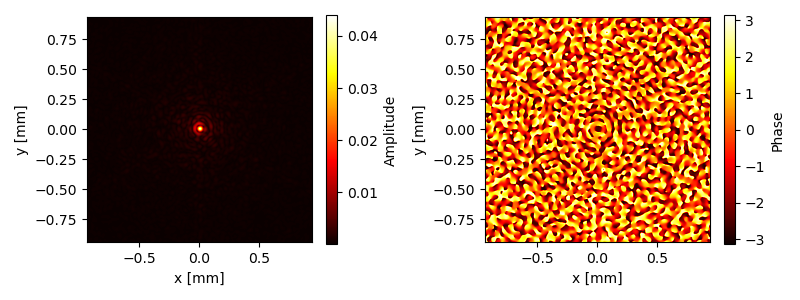
@@ -1,8 +1,16 @@
 import numpy as np
 import sys
-sys.path.insert(0, '/Users/joost/Dropbox/Werk/PhD/Analyses/Python/Analytical/Fourier Optics')
+sys.path.insert(0, '/Users/joost/Dropbox/Werk/PhD/Documents/Published/FourierOptics GitHub release/')
 from fourierOptics import *
 
+'''
+	Description:
+	This script generates a point spread function of the MICADO optical model.
+	During the setup a wavefront error of 200 nm RMS is added to the first 
+	prisms of the MICADO atmospheric dispersion corrector.
+'''
+
+
 if __name__ == '__main__':
 	# Initiate MICADO paraxial model
 	mcd = ParaxialMICADO()

demonstration scripts/generate_bahtinov_dispersion.py

@@ -1,9 +1,21 @@
 import numpy as np
 import sys
-sys.path.insert(0, '/Users/joost/Dropbox/Werk/PhD/Analyses/Python/Analytical/Fourier Optics')
+sys.path.insert(0, '/Users/joost/Dropbox/Werk/PhD/Documents/Published/FourierOptics GitHub release/')
 from fourierOptics import *
 
 
+'''
+	Description:
+	This script generates a point spread function of the MICADO optical model.
+	Here we apply a Bahtinov mask to the pupil and simulate a broadband PSF,
+	done through the summation of multiple (here: 15) wavelength slices. 
+	When there is atmospheric dispersion, the diffraction speckles created by the 
+	Bahtinov mask will start to point to a location outside the zeroth order 
+	PSF core.
+	Here, atmospheric dispersion is modelled as a wavelength dependent phase
+	tilt.
+'''
+
 if __name__ == '__main__':
 	# Initiate MICADO paraxial model
 	mcd = ParaxialMICADO()

demonstration scripts/generate_field.py

@@ -1,8 +1,17 @@
 import numpy as np
 import sys
-sys.path.insert(0, '/Users/joost/Dropbox/Werk/PhD/Analyses/Python/Analytical/Fourier Optics')
+sys.path.insert(0, '/Users/joost/Dropbox/Werk/PhD/Documents/Published/FourierOptics GitHub release/')
 from fourierOptics import *
-from pdb import set_trace
+
+
+'''
+	Description:
+	This script generates nine points in a small field to illustrate the 
+	most basic form of off-axis propagation. 
+	For larger off-axis distances the hx and hy values should directly
+	be supplied to the propagate function.
+'''
+
 
 def field_angle(hx, hy):
 	fx = hx * 0.0075
@@ -15,14 +24,6 @@ if __name__ == '__main__':
 	mcd = ParaxialMICADO()
 	wfe = WavefrontError(mcd.n, mcd.m)
 	
-	# Uncomment to load in WFE (coma)
-	# Problem here is that the field of view is too small to see 
-	# a radial effect...
-	# xin, yin = load_variable('../adc_data_coordinates.pkl')
-	# adcObj = ADC_surfaces(xin,yin)
-	# zern = wfe.zernike_cartesian([0,0,0,0,0,0,0,100e-5], adcObj.xz, adcObj.yz, rescale=False)
-	# mcd.ELT_ADC.p1.add_wavefront_error(zern)
-	
 	# Setup
 	l = 1.49e-3
 	Elist = []

demonstration scripts/generate_propagation_figures.py

@@ -1,9 +1,14 @@
 import numpy as np
 import sys
-sys.path.insert(0, '/Users/joost/Dropbox/Werk/PhD/Analyses/Python/Analytical/Fourier Optics')
+sys.path.insert(0, '/Users/joost/Dropbox/Werk/PhD/Documents/Published/FourierOptics GitHub release/')
 from fourierOptics import *
 import matplotlib.pyplot as plt
-from pdb import set_trace
+
+'''
+	Description:
+	This script generates the amplitude and phase information of all surfaces
+	in the MICADO paraxial model in a nicely presented form.
+'''
 
 if __name__ == '__main__':
 	plt.rc('font', family='serif')

demonstration scripts/thesis_propagation_figures.py

@@ -1,9 +1,16 @@
 import numpy as np
 import sys
-sys.path.insert(0, '/Users/joost/Dropbox/Werk/PhD/Analyses/Python/Analytical/Fourier Optics')
+sys.path.insert(0, '/Users/joost/Dropbox/Werk/PhD/Documents/Published/FourierOptics GitHub release/')
 from fourierOptics import *
 import matplotlib.pyplot as plt
-from pdb import set_trace
+
+'''
+	Description:
+	This script generates the amplitude and phase information of all surfaces
+	in the MICADO paraxial model in a nicely presented form.
+'''
+
+
 
 if __name__ == '__main__':
 	plt.rc('font', family='serif')
@@ -12,13 +19,10 @@ if __name__ == '__main__':
 	# Initiate MICADO paraxial model
 	mcd = ParaxialMICADO(n=3001, m=3001, dpix=50)
 
-	# Generate the PSF and plot it
-	# E, x, y = mcd.propagate(l=1.35e-3,surface=-1, zoom=True, show=True, save='all')
-
 	confList = [ ( 1, [-0.4, 0.4, -0.4, 0.4], 	'02_fourier_ELT-IFP.pdf'),
 				 ( 2, [-50, 50, -50, 50], 		'03_fourier_ELT-COL.pdf'),
 				 ( 4, [-50, 50, -50, 50], 		'04_fourier_ELT-MCD-ADC-P2.pdf'),
-				 (-1, [-1.2, 1.2, -1.2, 1.2], 	'05_fourier_ELT-MCD-DET.pdf')]
+				 (-1, [-1.2/2.669, 1.2/2.669, -1.2/2.669, 1.2/2.669], 	'05_fourier_ELT-MCD-DET.pdf')]
 
 
 	for i in range(len(confList)):
@@ -26,7 +30,7 @@ if __name__ == '__main__':
 		coordinates = confList[i][1]
 		savename = confList[i][2]
 		E, x, y = mcd.propagate(l=1.35e-3, surface=s, image_output=coordinates,
-								 zoom=False, show=False, save=savename)
+								 zoom=False, show=True, save=False)
 
 	Eout, x, y = mcd.propagate(l=1.35e-3, surface=0, zoom=False, show=False)
 	x /= 1e3 # convert to m
@@ -47,5 +51,5 @@ if __name__ == '__main__':
 	_ax2.set_ylabel('y [m]')
 	_fig.colorbar(_im2, ax=_ax2, label='Phase')
 	plt.tight_layout()
-	plt.savefig('01_fourier_ELT-M1.pdf', bbox_inches='tight', transparent=True)
+	# plt.savefig('01_fourier_ELT-M1.pdf', bbox_inches='tight', transparent=True)
-	plt.close()#show()
+	plt.show()

fourierOptics/__init__.py

@@ -3,9 +3,9 @@ from .fourier import *
 from .gaussian import *
 from .opticalTrain import *
 from .optics import *
+from .micado import *
 from .profiles import *
 from .psfFitter import *
 from .wavefrontErrors import *
 from .misc import *
-from .micado import *
 from .atmosphere import *

fourierOptics/atmosphere.py

@@ -1,6 +1,8 @@
 import numpy as np
 import scipy.special as spc
 from .misc import *
+import pyfftw
+import os
 
 '''
 	Various functions to simulate a seeing limited PSF. These functions are
@@ -53,6 +55,45 @@ def fried_r0(wvl, seeing):
 	return r0
 
 
+def r0converter(r0, lambda1, lambda2):
+	'''
+		Equivalent to anisocado.psf_utils.r0Converter()
+
+		Converts a r0 defined at some wavelength lambda1,
+		into a r0' at lambda2.
+		Lambda1 and 2 shall be in the SAME unit.
+		Returned r0 will be in the SAME unit than the input one.
+		Example::
+			r0_K = r0Converter(0.12, 500, 2200)
+	'''
+	return r0 * ( lambda2 / lambda1 )**( 6/5.)
+
+
+def r0_at_observed_zenith_distance(r0_at_zenith, zenith_distance):
+	'''
+		The seeing/r0 actually perceived by a telescope depends on the zenith
+		distance. This function converts a r0 given at zenith into the real r0
+		actually observed by the telescope.
+
+		Parameters:
+		-----------
+		r0_at_zenith    - Float or Array
+				Fried length r0 at zenith (degrees) in the wavelength of
+				interest. See also fried_r0() and r0converter().
+		zenith_distance - Float or Array. 
+				Observed zenith distance (degrees)
+
+		Returns:
+		r0 				- Float or Array
+				Observed r0 at the observed zenith distance
+		
+	'''
+	z = zenith_distance * np.pi / 180  # the same, in radians
+	r0 = r0_at_zenith * np.cos(z)**(3./5)
+	return r0
+
+
+
 def airmass(z):
 	'''
 		Converts zenith angle in degrees to airmass
@@ -83,7 +124,7 @@ def spectrum(k, r0, L0=25):
 	return spectrum 
 
 
-def add_seeing(wvl, sng, field_tuple):
+def add_seeing(wvl, sng, field_tuple, focal_length=3200):
 	'''
 		Computes the seeing limited PSF for a supplied amplitude
 		distribution.
@@ -96,6 +137,8 @@ def add_seeing(wvl, sng, field_tuple):
 			Atmospheric seeing in arcseconds.
 		field_tuple - Tuple 
 			Contains the PSF information (amplitude array, x coordinates, y coordinates)
+		focal_length - float
+			Focal length in mm of the telescope used.
 		
 		Returns:
 		psf_seeing 	- Array
@@ -105,8 +148,8 @@ def add_seeing(wvl, sng, field_tuple):
 	r01   = fried_r0(wvl, seeing=sng) * 1e3
 	A_psf, x_psf, y_psf = field_tuple
 	n,m = np.shape(x_psf)
-	fx = x_psf / (3200*wvl)
+	fx = x_psf / (focal_length*wvl)
-	fy = y_psf / (3200*wvl)
+	fy = y_psf / (focal_length*wvl)
 	dk = find_pixel_scale(fx)
 
 	# von-Karman spectrum of the atmosphere for the given frequencies in k-space
@@ -133,3 +176,398 @@ def add_seeing(wvl, sng, field_tuple):
 	return psf_seeing
 
 
+
+
+
+def add_scao(wvl, sng, field_tuple, focal_length=2059940, perfect_scao=False, 
+			dactu=540.3, offx=0, offy=0):
+	'''
+		After adding seeing, we would like to add Adaptive Optics to the system.
+		Based on the 'anisocado' package, I will try to reproduce an AO corrected
+		PSF for MICADO, with a nice seeing halo around it.
+
+		Some of the functions from anisocado will be reused or modified to make it
+		work for me.
+
+		Parameters
+		----------
+		wvl 		-	Float
+			Wavelength in mm corresponding to the supplied PSF
+		sng 		- 	Float
+			Atmospheric seeing in arcseconds.
+		field_tuple - Tuple 
+			Contains the PSF information (amplitude array, x coordinates, y coordinates)
+		focal_length - float
+			Focal length in mm of the telescope used.
+		perfect_scao - bool
+			Whether or not SCAO errors should be considered. If true, time delay,
+			anisoplanatism and others are added.
+		dactu 	- 	float
+			Distance between actuators on the DM in millimeters.
+		offx, offy - float
+			Angular offset in arcseconds from the SCAO guide star relative to the 
+			observed target. This will simulate anisoplanatism.
+		
+		Returns:
+		psf_seeing 	- Array
+			2D array containing the new seeing limited PSF information.
+
+	'''
+	L0 = 25*1e3 # outer scale parameter of the turbulence cells (in mm)
+	rms_wfe_mm = 100. * 1e-6 # Overall system wavefront error
+
+	r01   = fried_r0(wvl, seeing=sng) * 1e3
+	A_psf, x_psf, y_psf = field_tuple
+	n,m = np.shape(x_psf)
+	fx  = x_psf / (focal_length*wvl)
+	fy  = y_psf / (focal_length*wvl)
+	dk  = find_pixel_scale(fx)
+
+
+	# von-Karman spectrum of the atmosphere for the given frequencies in k-space
+	W_atm   = spectrum(np.hypot(fx.real, fy.real), r0=r01, L0=L0)
+	W_atm[int(n/2),int(m/2)] = 0
+
+	# M4 is the ELT deformable mirror that is used for SCAO
+	M4 = define_DM_FrequencyArea(fy, fx, dactu=dactu)
+
+	# [SKIPPED] W_aniso = anisoplanaticSpectrum(Cn2h, layerAltitude, L0, offx, offy, wvl, fx, fy, W_atm, M4)
+
+	# Assuming the correction is perfect within the controlled frequencies
+	W_fit = W_atm.copy()
+	W_fit[M4] = 0.0
+
+	if perfect_scao:
+		# Effect of isoplanatic errors
+		layerAltitude, Cn2h = get_Cn2h()
+		W_aniso = get_anisoplanatic_spectrum(Cn2h, layerAltitude, offx, offy, fx, fy, W_atm, M4)
+		
+		W_combined = W_fit + W_aniso
+
+
+	else:
+		# Alias effects, primarily at the edges of the DM
+		W_alias = get_aliasing_spectrum(fy, fx, r0=r01, L0=L0, M4=M4)
+
+		# Effect of isoplanatic errors
+		layerAltitude, Cn2h = get_Cn2h()
+		W_aniso = get_anisoplanatic_spectrum(Cn2h, layerAltitude, offx, offy, fx, fy, W_atm, M4)
+		
+		# Effect of something...
+		W_bp    = get_Bp_spectrum(fy, fx, W_atm=W_atm, DM=M4)
+		
+		# Effect of overall wavefront error contribution. Static.
+		W_other = get_wfe_spectrum(rms_wfe_mm, M4, dk, wvl)
+		
+		# W_aniso is so much smaller than all the other contributors!
+		W_combined = W_fit + W_aniso + W_alias + W_bp + W_other				   
+
+	# Compute the atmospheric OTF
+	# According to Roddier 1981, the atmospheric OTF can be derived from the phase structure function
+	# assuming that the phase is stationary accross the pupil and behaves as a Gaussian variable
+	# Bphi = np.fft.fft2(np.fft.ifftshift(W_combined))*dk**2
+	Bphi = fftw_forward(np.fft.ifftshift(W_combined))*dk**2
+	Dphi = np.fft.ifftshift((2 * (Bphi[0,0] - Bphi))) # ifftshift in Bphi en Dphi!
+	otf_ao = np.exp(-0.5*Dphi)
+
+	# Compute the OTF of the supplied PSF
+	# We can derive the OTF from the inverse Fourier transform of the PSF
+	psf = np.abs(A_psf)**2
+	otf_psf = np.fft.fftshift(fftw_inverse(np.fft.fftshift(psf)))
+	otf_psf = otf_psf/otf_psf.max()
+
+	# Compute the seeing-limited PSF
+	# Multiplication of OTF and then Fourier transform
+	otf  = otf_psf * otf_ao
+	psf_seeing = np.fft.fftshift(fftw_forward(np.fft.ifftshift(otf)))
+	return psf_seeing
+
+
+def define_DM_FrequencyArea(kx, ky, rotdegree=0, dactu=540.3):
+	'''
+		From anisocado.psf_utils.defineDmFrequencyArea()
+
+		<kx>        : spatial frequency produced by the
+					  function computeSpatialFreqArrays() (metres^-1)
+		<ky>        : idem kx
+		<rotdegree> : rotation of M4 (degrees)
+		<dactu>     : value of actuator pitch of M4 (metres)
+		
+		The function returns the 2D domain of spatial frequencies which can be
+		impacted by M4, i.e. the M4 compensation domain.
+		Underlying assumtions are than M4 is of an hexagonal pattern, with an
+		inter-actuator distance <dactu> set by default to 54.03 cm (=540.3 mm).
+		Result is returned with a frequency corner-centred representation.
+	'''
+
+	# cut-off frequency
+	fc = (1./np.sqrt(3)) / dactu
+
+	# mask frequency definition
+	A = np.pi/3  # 60 degrees
+	A0 = rotdegree * np.pi / 180
+	msk = np.abs(np.cos(A0)*ky+np.sin(A0)*kx)<fc
+	msk = np.logical_and(msk, np.abs(np.cos(A+A0)*ky+np.sin(A+A0)*kx)<fc)
+	msk = np.logical_and(msk, np.abs(np.cos(2*A+A0)*ky+np.sin(2*A+A0)*kx)<fc)
+	k = np.sqrt(kx**2 + ky**2)
+	msk = np.logical_and(msk, k < (fc*1.115))
+	return msk
+
+
+def get_aliasing_spectrum(kx, ky, r0, L0, M4, dssp=0.4015):
+	'''
+		All units scale with millimeter (either in mm^-1 or mm)	
+	'''
+	# convert dssp from meters to millimeters
+	dssp *= 1e3
+	ke = 1.0 / dssp  # computes the sampling spatial-frequency of the WFS
+
+	kxt = kx[M4]
+	kyt = ky[M4]
+	Wt  = ((kxt-ke)**2 + kyt**2 + 1./L0**2.)**(-11./6)
+	Wt += ((kxt+ke)**2 + kyt**2 + 1./L0**2.)**(-11./6)
+	Wt += (kxt**2 + (kyt-ke)**2 + 1./L0**2.)**(-11./6)
+	Wt += (kxt**2 + (kyt+ke)**2 + 1./L0**2.)**(-11./6)
+	Wt *= 0.0228956 * r0**(-5./3)
+	Walias = np.zeros(M4.shape)
+	Walias[M4] = Wt.real
+
+	return Walias
+
+
+def get_anisoplanatic_spectrum(Cn2h, layerAltitude, offx, offy,
+						  kx, ky, atm_psd, DM):
+	'''
+	From anisocado.psf_utils.anisoplanaticSpectrum(), modified to accomodate
+	length in millimeters, i.s.o. meters.
+
+	<Cn2h>          : list of normalised (np.sum(Cn2h)==1.0) strengh of
+					  turbulence of each layer (no unit)
+	<layerAltitude> : list of altitudes of the turbulence layers (metres)
+	<L0>            : value of the outer scale (metres)
+	<offx>          : off-axis distance of the star along X axis (arcsec)
+	<offy>          : idem along Y axis (arcsec)
+	<wavelength>    : wavelength (metres)
+	<kx>            : spatial frequency produced by
+					  the function computeSpatialFreqArrays() (metres^-1)
+	<ky>            : idem kx
+	<atm_psd>      : turbulent spectrum from function computeWiener()
+	<DM>            : frequency domain of M4 (boolean) computed by the
+					  function M4 = defineDmFrequencyArea(kx, ky, 0)
+	Computes the phase spectrum (spatial frequencies) contribution due to the
+	anisoplanatism in the AO compensation for a source located off-axis from
+	the SCAO guide star by some amount (offx, offy).
+	In input, the distribution of the turbulence in altitude is given.
+	Result is returned with a frequency corner-centred representation.
+	'''
+
+	# number of turbulent layers involved in that computation
+	nlayers = len(Cn2h)
+
+	# conversion arcsec to radians
+	RASC = 206264.8062471
+
+	# prepare memory alloc for transfer function of anisoplanatism
+	Haniso = np.zeros(kx.shape)
+
+	# loop over turbulent layers, summing transfer function of each layer
+	for i in range(nlayers):
+		dx = layerAltitude[i] * offx / RASC # shift in millimetres on the layer in X
+		dy = layerAltitude[i] * offy / RASC # idem, in Y
+		tmp = (2j*np.pi*dx)*kx + (2j*np.pi*dy)*ky
+		Haniso += Cn2h[i] * np.abs(1 - np.exp( tmp ))**2
+
+	# now applying the transfer function on the Wiener spectrum, only in the
+	# spatial frequency range of M4
+	Waniso = np.zeros(Haniso.shape)
+	Waniso[DM] = Haniso[DM] * atm_psd[DM]
+
+	return Waniso
+
+
+def get_Bp_spectrum(kx, ky, W_atm, DM, V=10, Fe=500, tret=4e-3, gain=0.3):
+	'''
+		From anisocado.psf_utils.computeBpSpectrum()
+
+		V = 10. 	 - Wind speed in m/s
+		Fe = 500. Hz - response rate
+		tret = 0.004 - time delay in seconds
+		gain = 0.3   - gain of the control loop
+		f = computeBpSpectrum(kx, ky, V, Fe, tret, gain, W, M4)
+	'''
+	k = np.sqrt(kx*kx + ky*ky)
+	nu = k * V / np.sqrt(2)
+	Wbp = hcor(nu, Fe, tret, gain, 500) * W_atm
+	Wbp[np.logical_not(DM)] = 0.
+	return Wbp
+
+
+def hcor(freq, Fe, tret, G, BP, an=True):
+	'''
+	From anisocado.psf_utils.hcor()
+
+	***** Fonction extraite de STYC le 9 Jan 2013 *****
+	The option an=1 sets the integrator to "analog". Doing this, an
+	extra 1/2 frame delay is added compared to case of the numeric
+	integrator an=0.
+	<tret> is the delay expressed as a *time in seconds*, between the
+	end of the integration and the start of the command.
+	'''
+
+	Te = 1. / Fe
+	p = 1j * 2 * np.pi * freq + 1e-12
+
+	Hint = 1./(1-np.exp(-p*Te)) 		# numeric integrator
+	Hccd = (1.-np.exp(-p*Te))/(p*Te)  	# echant bloqueur avec retard 1/2 trame
+	Hdac = Hccd                    		# echant bloqueur avec retard 1/2 trame
+	Hret = np.exp(-p*tret)
+	Hmir = 1./(1. + 1j*freq/BP)
+	Hbo = Hint * Hccd * Hdac * Hret * Hmir
+	Hcor   = 1./abs(1 + Hbo*G)**2
+	return Hcor
+
+
+def get_wfe_spectrum(wfe_rms, M4, uk, wavelength):
+	'''
+		<nmRms>  : number of nm rms
+		<M4>     : frequency domain of M4 (boolean) computed by the
+						  function M4 = defineDmFrequencyArea(kx, ky, 0)
+		<uk> : # size of the 'spatial frequency pixel' in m^-1
+		<wavelength>    : wavelength (metres)
+		Example::
+			N = 512
+			pixelSize = 4.2
+			L0 = 25.0
+			offx, offy = (34., 12.)
+			wavelength = 1.65e-6
+			kx, ky, uk = computeSpatialFreqArrays(N, pixelSize, wavelength)
+			M4 = defineDmFrequencyArea(kx, ky, 0)
+			nmRms = 250.
+			f = otherSpectrum(nmRms, M4, uk, wavelength)
+	'''
+	fact = 2 * np.pi * wfe_rms / uk / wavelength
+	fact = fact**2
+	tot = np.sum(M4)
+	Wothers = np.zeros(M4.shape)
+	Wothers[M4] = fact / tot
+
+	return Wothers
+
+
+
+def get_Cn2h(myProfile='EsoMedian'):
+	'''
+	From anisocado.psf_utils.get_atmospheric_turbulence()
+
+	Returns the relative level of turbulence at a given height
+	Note: The np.sum(Cn2h) = 1.0
+	Turbulence profile have been taken from ESO-258292: "Relevant Atmospheric
+	Parameters for E-ELT AO Analysis and Simulations".
+	The following 3 turbulence profile are currently available:
+	* ``EsoQ1``
+		Best atmospheric conditions - First Quartile Armazones atmospheric
+		turbulence profile
+	* ``EsoMedian`` [also ``officialEsoMedian``]
+		Median atmospheric conditions - Median Armazones atmospheric turbulence
+		profile
+	* ``EsoQ4``
+		Worst atmospheric conditions - First Quartile Armazones atmospheric
+		turbulence profile
+	Additional turbulence profiles include:
+	* ``oldEso``
+		The old ESO profile from before 2010. Cn2h paramateres are taken from
+		ref. E-SPE-ESO-276-0206_atmosphericparameters
+	* ``gendron``
+		The Gendron profile. Short, fast. Saves CPU. Carbon efficient.
+		The np.sum(Cn2h) = 1.0 is hyper-guaranteed here.
+	
+	Parameters
+	----------
+	myProfile : str, optional
+		Profile name: ['EsoQ1', 'EsoMedian', 'EsoQ4', 'oldEso', 'gendron']
+	
+	Returns
+	-------
+	layerAltitude : list of floats
+		[m] height of layer above ground
+	Cn2h : list of floats
+		Relative strength of turbulence
+	'''
+
+	layerAltitude, Cn2h = [], []
+
+	if myProfile == 'oldEso':
+		layerAltitude = [47., 140, 281, 562, 1125, 2250, 4500, 9000, 18000.]
+		Cn2h = [0.5224, 0.026, 0.0444, 0.116, 0.0989,
+				0.0295, 0.0598, 0.043, 0.06]
+
+	elif myProfile == 'officialEsoMedian' or myProfile == 'EsoMedian' :
+		layerAltitude = [30, 90, 150, 200, 245, 300, 390, 600, 1130, 1880, 2630,
+						 3500, 4500, 5500, 6500, 7500, 8500, 9500, 10500, 11500,
+						 12500, 13500, 14500, 15500, 16500, 17500, 18500, 19500,
+						 20500, 21500, 22500, 23500, 24500, 25500, 26500]
+		Cn2h = [24.2, 12, 9.68, 5.9, 4.73, 4.73, 4.73, 4.73, 3.99, 3.24, 1.62,
+				2.6, 1.56, 1.04, 1, 1.2, 0.4, 1.4, 1.3, 0.7, 1.6, 2.59, 1.9,
+				0.99, 0.62, 0.4, 0.25, 0.22, 0.19, 0.14, 0.11, 0.06, 0.09, 0.05,
+				0.04]
+		Cn2h = np.array(Cn2h)
+		Cn2h /= np.sum(Cn2h)
+
+	elif myProfile == 'EsoQ1':
+		layerAltitude = [30, 90, 150, 200, 245, 300, 390, 600, 1130, 1880, 2630,
+						 3500, 4500, 5500, 6500, 7500, 8500, 9500, 10500, 11500,
+						 12500, 13500, 14500, 15500, 16500, 17500, 18500, 19500,
+						 20500, 21500, 22500, 23500, 24500, 25500, 26500]
+		Cn2h = [22.6, 11.2, 10.1, 6.4, 4.15, 4.15, 4.15, 4.15, 3.1, 2.26, 1.13,
+				2.21, 1.33, 0.88, 1.47, 1.77, 0.59, 2.06, 1.92, 1.03, 2.3, 3.75,
+				2.76, 1.43, 0.89, 0.58, 0.36, 0.31, 0.27, 0.2, 0.16, 0.09, 0.12,
+				0.07, 0.06]
+		Cn2h = np.array(Cn2h)
+		Cn2h /= np.sum(Cn2h)
+
+	elif myProfile == 'EsoQ4':
+		layerAltitude = [30, 90, 150, 200, 245, 300, 390, 600, 1130, 1880, 2630,
+						 3500, 4500, 5500, 6500, 7500, 8500, 9500, 10500, 11500,
+						 12500, 13500, 14500, 15500, 16500, 17500, 18500, 19500,
+						 20500, 21500, 22500, 23500, 24500, 25500, 26500]
+		Cn2h = [23.6, 13.1, 9.81, 5.77, 6.58, 6.58, 6.58, 6.58, 5.4, 3.2, 1.6,
+				2.18, 1.31, 0.87, 0.37, 0.45, 0.15, 0.52, 0.49, 0.26, 0.8, 1.29,
+				0.95, 0.49, 0.31, 0.2, 0.12, 0.1, 0.09, 0.07, 0.06, 0.03, 0.05,
+				0.02, 0.02]
+		Cn2h = np.array(Cn2h)
+		Cn2h /= np.sum(Cn2h)
+
+	elif myProfile == 'gendron':
+		Cn2h = [1.0]
+		layerAltitude = [4414.]
+
+	layerAltitude = (np.asarray(layerAltitude) * 1e3).tolist()
+	return layerAltitude, Cn2h
+
+
+def fftw_forward(Ain):
+	# Initialization of input array
+	_A_in 		= pyfftw.empty_aligned(Ain.shape, dtype='complex128')
+	_A_in[:] 	= Ain
+
+	# Initialization of output array
+	_A_out 		= pyfftw.empty_aligned(Ain.shape, dtype='complex128')
+
+	# Invoking Pythors FFTW
+	_FFTW_Obj 	= pyfftw.FFTW( _A_in, _A_out, axes=(0,1), direction='FFTW_FORWARD', threads=os.cpu_count(), flags=('FFTW_ESTIMATE',))
+	_FFTW_Obj()
+	return _A_out
+
+def fftw_inverse(Ain):
+	# Initialization of input array
+	_A_in 		= pyfftw.empty_aligned(Ain.shape, dtype='complex128')
+	_A_in[:] 	= Ain
+
+	# Initialization of output array
+	_A_out 		= pyfftw.empty_aligned(Ain.shape, dtype='complex128')
+
+	# Invoking Pythors FFTW
+	_FFTW_Obj 	= pyfftw.FFTW( _A_in, _A_out, axes=(0,1), direction='FFTW_BACKWARD', threads=os.cpu_count(), flags=('FFTW_ESTIMATE',))
+	_FFTW_Obj()
+	return _A_out
+

fourierOptics/fourier.py

@@ -6,6 +6,7 @@ from scipy.optimize import leastsq
 from matplotlib.ticker import FormatStrFormatter
 from matplotlib.colors import LogNorm
 import pyfftw
+import os
 from .misc import find_pixel_scale
 
 class FourierOptics:
@@ -68,7 +69,7 @@ class FourierOptics:
 		_E_xy0[:] 	= np.fft.ifftshift(A)  					# use ifftshift to shift origin to start array
 		_IntensityNormFactor = np.sum(np.abs(_E_xy0)**2)	# Factor to scale the intensity after the FFTs
 		_Az0 		= pyfftw.empty_aligned((_n,_m), dtype='complex128')
-		_FFTW_Obj 	= pyfftw.FFTW( _E_xy0, _Az0, axes=(0,1), direction='FFTW_BACKWARD', threads=6, flags=('FFTW_ESTIMATE',))
+		_FFTW_Obj 	= pyfftw.FFTW( _E_xy0, _Az0, axes=(0,1), direction='FFTW_BACKWARD', threads=os.cpu_count(), flags=('FFTW_ESTIMATE',))
 		_FFTW_Obj()
 
 		# E-field at z=dz is the fourier transform of A(z=0)*e^(-ikz)
@@ -86,7 +87,7 @@ class FourierOptics:
 		_A_in 		= pyfftw.empty_aligned((_n,_m), dtype='complex128')
 		_A_in[:] 	= _Az0 * _phaseFactor
 
-		_FFTW_Obj2 	= pyfftw.FFTW( _A_in, _E_xyz, axes=(0,1), direction='FFTW_FORWARD', threads=6, flags=('FFTW_ESTIMATE',))
+		_FFTW_Obj2 	= pyfftw.FFTW( _A_in, _E_xyz, axes=(0,1), direction='FFTW_FORWARD', threads=os.cpu_count(), flags=('FFTW_ESTIMATE',))
 		_FFTW_Obj2()
 		_E_xyz 		= np.fft.fftshift(_E_xyz) 				# use fftshift to move the origin from edge to center
 		_E_xyz /= np.sqrt(_IntensityNormFactor) 			# Normalization back to initial energy.
@@ -213,7 +214,7 @@ class FourierOptics:
 		
 		# Output of the FFT evaluated at frequency fx = x / (lambda * z)
 		_U_out 			= pyfftw.empty_aligned((_n,_m), dtype='complex128')
-		_FFTW_Obj		= pyfftw.FFTW( np.fft.ifftshift(_U_in), _U_out, axes=(0,1), direction='FFTW_FORWARD', threads=6, flags=('FFTW_ESTIMATE',))
+		_FFTW_Obj		= pyfftw.FFTW( np.fft.ifftshift(_U_in), _U_out, axes=(0,1), direction='FFTW_FORWARD', threads=os.cpu_count(), flags=('FFTW_ESTIMATE',))
 		_FFTW_Obj()
 		_U_out 			= np.fft.fftshift(_U_out)
 
@@ -365,7 +366,7 @@ class FourierOptics:
 		
 		# Output of the FFT
 		_A_out 			= pyfftw.empty_aligned(PSF.shape, dtype='complex128')
-		_FFTW_Obj		= pyfftw.FFTW( np.fft.ifftshift(_A_in), _A_out, axes=(0,1), direction='FFTW_FORWARD', threads=6, flags=('FFTW_ESTIMATE',))
+		_FFTW_Obj		= pyfftw.FFTW( np.fft.ifftshift(_A_in), _A_out, axes=(0,1), direction='FFTW_FORWARD', threads=os.cpu_count(), flags=('FFTW_ESTIMATE',))
 		_FFTW_Obj()
 		_A_out 			= np.fft.fftshift(_A_out)
 

fourierOptics/micado.py

@@ -9,7 +9,16 @@ from .wavefrontErrors import *
 from .misc import *
 
 
+'''
+Changelog:
 
+Changes w.r.t. the old MICADO paraxial model:
+- Changed focal length of collimator lens from 4278.32701 to 1601.688 mm
+- Changed distance from ADC to collimator lens from 50 mm to 74 mm.
+- Changed thickness of ADC prisms from 25 to 15 mm
+- Changed working F-number (WFNO) from 53.4466 to 20.0269
+- This results in a change of the plate scale from 0.1001 arcsec/mm to 0.2672 arcsec/mm
+'''
 
 class ParaxialMICADO:
 	def __init__(self, l=1.35e-3, n=1001, m=1001, dpix=160, entrance_pupil='ELT'):
@@ -32,7 +41,7 @@ class ParaxialMICADO:
 		self.ELT_FP			= OpticalSurface(name='MCD-IFP')
 		self.ELT_COL		= ParaxialLens(CA=154.54, f=1418.94, name='MCD-COL')
 		self.ELT_ADC 		= ADCObject()
-		self.ELT_CAM		= ParaxialLens(CA=89.2, f=4278.32701, name='MCD-CAM')
+		self.ELT_CAM		= ParaxialLens(CA=89.2, f=1601.688, name='MCD-CAM')
 		self.ELT_DET		= OpticalSurface(name='MCD-DET')
 
 		# Built optical train
@@ -41,11 +50,12 @@ class ParaxialMICADO:
 		self.MCD.add_object(self.ELT_FP, 		dist=self.ELT_MIRROR.f)
 		self.MCD.add_object(self.ELT_COL, 		dist=self.ELT_COL.f)
 		self.ELT_ADC.add_to_optical_train(self.MCD, 1209.4718)
-		self.MCD.add_object(self.ELT_CAM, 		dist=50)
+		self.MCD.add_object(self.ELT_CAM, 		dist=74)
 		self.MCD.add_object(self.ELT_DET, 		dist=self.ELT_CAM.f)
 
 		self.last_PSF 		= None
 		self.clean_PSF 		= None
+		self.pixelscale 	= 4e-3 # arcseconds/pixel
 		self.platescale 	= self.set_plate_scale()
 		print ('Your resolution is {}x{} with a pixel size of {}'.format(self.n,self.m,self.dpix))
 		print('This means your grid is {} mm by {} mm, with each pixel {} mm.'.format(
@@ -233,6 +243,8 @@ class ParaxialMICADO:
 			elif surfaces[s] == self.ELT_FP:
 				if print_progress: print('Propagating from ELT-IFP to MCD-COL')
 				Ein = Eout
+				if self.ELT_FP.wavefrontError:
+					Ein *= self.ELT_FP.phase_delay(x, y, l, ip_type='phase')
 				Eout, x, y = fou.fresnel_propagation(Ein, x, y, dz=self.ELT_COL.f, oversample=None, 
 					show=show[s], save=saveList[s], outputCoordinates=output_coordinates[s], 
 					apply_interpolation=apply_ip[s], tx=tilt_x[s], ty=tilt_y[s])
@@ -332,7 +344,7 @@ class ParaxialMICADO:
 								[-120, 120, -120, 120],
 								[-120, 120, -120, 120],
 								[-120, 120, -120, 120],
-								[-2.5, 2.5, -2.5, 2.5]
+								[-2.5/2.669, 2.5/2.669, -2.5/2.669, 2.5/2.669]
 							  ]
 		elif coordinates is not None:
 			_coordinatesList = coordinates
@@ -384,12 +396,12 @@ class ParaxialMICADO:
 			_apply_ip[surf] = True
 		return _apply_ip
 
-	def set_plate_scale(self):
+	def set_plate_scale(self, wfno=20.0269):
 		'''
 			Returns the platescale of this paraxial MICADO
 			model in arcseconds/mm.
 		'''
-		_ps = (3600*180/np.pi) / (self.ELT_MIRROR.CA * 53.4466)
+		_ps = (3600*180/np.pi) / (self.ELT_MIRROR.CA * wfno)
 		self.platescale = _ps
 		return _ps
 
@@ -522,7 +534,7 @@ class ParaxialMICADO:
 										a2y=np.deg2rad(self.ELT_ADC.p4.tilt2y),
 										n_glass=self.ELT_ADC.p4.find_refractive_index(self.l, unit='millimeter'))
 		positions_and_angles.append([xp,yp,np.degrees(tx),np.degrees(ty)])
-		xp, yp, tx,ty = get_free_space_propagation_rtm(xp,yp,tx,ty,50)
+		xp, yp, tx,ty = get_free_space_propagation_rtm(xp,yp,tx,ty,74)
 
 		# ELT-MCD-CAM:
 		xp, yp, tx, ty = get_paraxial_lens_rtm(xp, yp, tx, ty, self.ELT_CAM.f, self.ELT_CAM.f)
@@ -546,8 +558,8 @@ class ParaxialMICADO:
 							6.84022e5+1418.94+1209.4718 + 15 + 1 + 15 + 8 + 15, # ADC p3
 							6.84022e5+1418.94+1209.4718 + 15 + 1 + 15 + 8 + 15 + 1, # Between p3 and p4
 							6.84022e5+1418.94+1209.4718 + 15 + 1 + 15 + 8 + 15 + 1 + 15, # ADC p4
-							6.84022e5+1418.94+1209.4718 + 15 + 1 + 15 + 8 + 15 + 1 + 15 + 50, # MCD-CAM
+							6.84022e5+1418.94+1209.4718 + 15 + 1 + 15 + 8 + 15 + 1 + 15 + 74, # MCD-CAM
-							6.84022e5+1418.94+1209.4718 + 15 + 1 + 15 + 8 + 15 + 1 + 15 + 50 + 4278.32701 # Focal plane
+							6.84022e5+1418.94+1209.4718 + 15 + 1 + 15 + 8 + 15 + 1 + 15 + 74 + 1601.688 # Focal plane
 							])
 		return x_out, y_out, tx_out, ty_out, z_out
 
@@ -640,7 +652,7 @@ class ParaxialMICADO:
 		# Fourth prism
 		xp, yp, tx,ty = get_free_space_propagation_rtm(xp,yp,tx,ty,self.ELT_ADC.p4.thickness)
 		positions_and_angles.append([xp,yp,np.degrees(tx),np.degrees(ty)])
-		xp, yp, tx,ty = get_free_space_propagation_rtm(xp,yp,tx,ty,50)
+		xp, yp, tx,ty = get_free_space_propagation_rtm(xp,yp,tx,ty,74)
 
 		# ELT-MCD-CAM:
 		xp, yp, tx, ty = get_paraxial_lens_rtm(xp, yp, tx, ty, self.ELT_CAM.f, self.ELT_CAM.f)
@@ -664,8 +676,8 @@ class ParaxialMICADO:
 							6.84022e5+1418.94+1209.4718 + 15 + 1 + 15 + 8 + 15, # ADC p3
 							6.84022e5+1418.94+1209.4718 + 15 + 1 + 15 + 8 + 15 + 1, # Between p3 and p4
 							6.84022e5+1418.94+1209.4718 + 15 + 1 + 15 + 8 + 15 + 1 + 15, # ADC p4
-							6.84022e5+1418.94+1209.4718 + 15 + 1 + 15 + 8 + 15 + 1 + 15 + 50, # MCD-CAM
+							6.84022e5+1418.94+1209.4718 + 15 + 1 + 15 + 8 + 15 + 1 + 15 + 74, # MCD-CAM
-							6.84022e5+1418.94+1209.4718 + 15 + 1 + 15 + 8 + 15 + 1 + 15 + 50 + 4278.32701 # Focal plane
+							6.84022e5+1418.94+1209.4718 + 15 + 1 + 15 + 8 + 15 + 1 + 15 + 74 + 1601.688 # Focal plane
 							])
 		return x_out, y_out, tx_out, ty_out, z_out
 

fourierOptics/micado_old.py

@@ -0,0 +1,798 @@
+import numpy as np
+from .fourier import *
+from .gaussian import *
+from .opticalTrain import *
+from .optics import *
+from .profiles import *
+from .psfFitter import *
+from .wavefrontErrors import *
+from .misc import *
+
+
+
+
+class ParaxialMICADO:
+	def __init__(self, l=1.35e-3, n=1001, m=1001, dpix=160, entrance_pupil='ELT'):
+		self.l 				= l
+		self.dpix 			= dpix
+		self.n, self.m 		= n, m
+		self.x, self.y 		= np.meshgrid(np.linspace(-n/2*dpix, n/2*dpix, n), np.linspace(-m/2*dpix, m/2*dpix, m))	
+		if entrance_pupil == 'ELT':
+			self.ELT_MASK 		= Profiles().ELT_pupil(n,m,dpix).astype('complex128')
+		elif entrance_pupil == 'obscured':
+			r1 = 38542/2
+			r2 = 10700/2
+			self.ELT_MASK 		= Profiles().obscured_top_hat(r1, r2, n, m, dpix).astype('complex128')
+		elif entrance_pupil == 'open':
+			r1 = 38542/2
+			self.ELT_MASK 		= Profiles().top_hat(r1, n, m, dpix).astype('complex128')
+
+		# Built optical system elements
+		self.ELT_MIRROR 	= ParabolicMirror(dx=0, dy=0, name='ELT-paraxial', CA=38542, f=6.84022e5)	
+		self.ELT_FP			= OpticalSurface(name='MCD-IFP')
+		self.ELT_COL		= ParaxialLens(CA=154.54, f=1418.94, name='MCD-COL')
+		self.ELT_ADC 		= ADCObject()
+		self.ELT_CAM		= ParaxialLens(CA=89.2, f=4278.32701, name='MCD-CAM')
+		self.ELT_DET		= OpticalSurface(name='MCD-DET')
+
+		# Built optical train
+		self.MCD 			= OpticalTrain()
+		self.MCD.add_object(self.ELT_MIRROR, 	dist=0)
+		self.MCD.add_object(self.ELT_FP, 		dist=self.ELT_MIRROR.f)
+		self.MCD.add_object(self.ELT_COL, 		dist=self.ELT_COL.f)
+		self.ELT_ADC.add_to_optical_train(self.MCD, 1209.4718)
+		self.MCD.add_object(self.ELT_CAM, 		dist=50)
+		self.MCD.add_object(self.ELT_DET, 		dist=self.ELT_CAM.f)
+
+		self.last_PSF 		= None
+		self.clean_PSF 		= None
+		self.pixelscale 	= 4e-3 # arcseconds/pixel
+		self.platescale 	= self.set_plate_scale()
+		print ('Your resolution is {}x{} with a pixel size of {}'.format(self.n,self.m,self.dpix))
+		print('This means your grid is {} mm by {} mm, with each pixel {} mm.'.format(
+			self.x.max()-self.x.min(), self.y.max()-self.y.min(), self.dpix))
+
+
+	def apply_mask(self, mask, replace=True):
+		'''
+			Set a mask to the ELT entrance pupil.
+		'''
+		if replace:
+			self.ELT_MASK = mask.astype('complex128')
+		elif not replace:
+			self.ELT_MASK *= mask
+
+
+	def set_PSF(self, PSF, x, y, perfect=True):
+		'''
+			If calculating another PSF takes to long,
+			one can set a custom PSF using this 
+			function.
+
+			Can be set as the 'clean' PSF or as another
+			'last' PSF, with the perfect flag.
+		'''
+		if perfect:
+			self.clean_PSF = (PSF, x, y)
+		elif not perfect:
+			self.last_PSF  = (PSF, x, y)
+
+
+	def centroid_shift(self, method='Coupling', reference_PSF=None, **kwargs):
+		'''
+			Do a centroid shift calculation for the given method.
+			This is a quick way of doing it. It only returns the 
+			centroid shift (and uncertainties) and no other parameters.
+		'''
+		assert (self.last_PSF is not None), 'PSF necessary for fitting.'
+		if 'initialGuess' in kwargs:
+			guess_value = kwargs.get('initialGuess')
+
+		if reference_PSF is None:
+			PSF, x, y = self.last_PSF
+		elif reference_PSF is not None:
+			PSF, x, y = reference_PSF
+		fitter = PSFFitter(x.real,y.real,np.abs(PSF)**2)
+
+		if method == 'Coupling':
+			assert (self.clean_PSF is not None), 'Perfect PSF necessary for comparison.'
+			Eclean, xclean, yclean = self.clean_PSF
+			fitted_PSF, popt, var, coupling = fitter.fit_custom_field(Eclean, PSF, return_coupling=True, **kwargs)
+			x0, y0 		= np.asarray(popt).T
+			sx0, sy0 	= np.asarray(np.sqrt(var)).T
+			return x0, y0, sx0, sy0, coupling
+
+		elif method == 'Airy':
+			if 'initialGuess' not in kwargs:
+				guess_value = (0.03**2, 0.0, 0.0, 0.0, 0.03)
+			fitted_PSF, popt, pcov = fitter.fit_airy_PSF(initialGuess=guess_value)
+			_, x0, y0, _, _ = popt
+			pcov_list = [ np.sqrt(pcov[i][i]) for i in range(len(pcov)) ]
+			_, sx0, sy0, _, _ = np.asarray(pcov_list).T
+
+		elif method == 'Obscured Airy':
+			if 'initialGuess' not in kwargs:
+				guess_value = (0.03**2, 0.0, 0.0, 0.0, 0.03)
+			fitted_PSF, popt, pcov = fitter.fit_fixed_obscuration_airy_PSF(initialGuess=guess_value)
+			_, x0, y0, _, _ = popt
+			pcov_list = [ np.sqrt(pcov[i][i]) for i in range(len(pcov)) ]
+			_, sx0, sy0, _, _ = np.asarray(pcov_list).T
+
+		elif method == 'Gaussian':
+			if 'initialGuess' not in kwargs:
+				guess_value = (0.04, 0, 0, 0.01, 0.01, 0, 0)
+			fitted_PSF, popt, pcov = fitter.fit_gaussian_PSF(initialGuess=guess_value)
+			_, x0, y0, _, _, _, _ = popt
+			pcov_list = [ np.sqrt(pcov[i][i]) for i in range(len(pcov)) ]
+			_, sx0, sy0, _, _, _, _ = np.asarray(pcov_list).T
+
+		elif method == 'Moffat':
+			if 'initialGuess' not in kwargs:
+				guess_value = (0.04, 0, 0, 0.01, 0.01, 0, 0, 4)
+			fitted_PSF, popt, pcov = fitter.fit_moffat_PSF(initialGuess=guess_value)
+			_, x0, y0, _, _, _, _, _ = popt
+			pcov_list = [ np.sqrt(pcov[i][i]) for i in range(len(pcov)) ]
+			_, sx0, sy0, _, _, _, _, _ = np.asarray(pcov_list).T
+
+		elif method == 'Barycenter':
+			x0, y0, sx0, sy0 = fitter.fit_barycenter(amplitude=False)
+
+		return x0, y0, sx0, sy0
+
+
+	def propagate(self, l=None, surface=-1, zoom=False, hx=0, hy=0, load_up_to_adc=None, 
+		coordinates=None, show=False, image_output=None, save=None, apply_interpolation=True, 
+		print_progress=True, defocus=None):
+		'''
+			Propagate the input wavefront through the MICADO paraxial
+			model. Optionally the propagation starts at the ADC, if 
+			a data file with the wavefront at that point is defined.
+
+			Parameters:
+			l 				- Desired wavelength of the propagation
+			surface 		- Surface to propagate to. Default: -1 = Detector plane
+			zoom 			- Zoom in on the PSF on the detector?
+			load_up_to_adc 	- Use a .pkl file to load in the wavefront just before the adc.
+			coordinates 	- User defined coordinates that define the propagation sampling.
+			show_final 		- Plots the final amplitude and phase if True.
+
+			Returns:
+			Exyz 			- Complex field with shape n,m describing the amplitude and phase
+							  of the wavefront at the output surface.
+			x, y 			- Corresponding x and y coordinates, in mm.
+		'''
+		# Set up wavelength
+		l = self.l if not l else l
+	
+		# Setting up the arguments for each surface propgation
+		surfaces 			= self.get_surfaces()
+		surface 			= len(surfaces)-1 if surface == -1 else surface
+		coordinatesList 	= self.get_coordinates(coordinates)
+		show,show_final_zoom= self.get_show_image(show, zoom, len(surfaces), surface)
+		output_coordinates 	= self.get_image_coordinates(image_output, coordinatesList, len(surfaces), surface)
+		saveList 			= self.get_save_image(save, len(surfaces), surface)
+		apply_ip 			= self.get_image_interpolation(apply_interpolation, zoom, len(surfaces), surface)
+		tilt_x, tilt_y		= self.get_tilt_angles(hx, hy)
+
+		# Set up the FourierOptics object for propagation
+		fou = FourierOptics(l=l)
+		x, y = self.x, self.y
+		p = 1 # Used as counter for the ADC prisms.
+		
+		# Load the data up to the ADC (useful for many iterations on the same 
+		# calculation, where differences only appear at or after the ADC)
+		if load_up_to_adc is not None:
+			Eout, x, y = load_variable(load_up_to_adc)
+			x = x.real
+			y = y.real
+			s = 4
+		elif load_up_to_adc is None:
+			s = 0
+
+		# Start propgation
+		if print_progress: print('Starting propagation...')
+		while s <= surface:
+			if (surfaces[s] == self.ELT_MASK).all():
+				Ein  = surfaces[s]
+				Eout = surfaces[s]
+				if show[s] or saveList[s]:
+					_fig = plt.figure(figsize=(8,3))
+					_ax = _fig.add_subplot(121)
+					_im = _ax.imshow(np.abs(Eout), cmap='hot', extent=[x.min(), x.max(), y.min(), y.max()])
+					_ax.set_xlim([x.min(), x.max()])
+					_ax.set_ylim([y.min(), y.max()])
+					_ax.set_xlabel('x [mm]')
+					_ax.set_ylabel('y [mm]')
+					_fig.colorbar(_im, ax=_ax, label='Amplitude')
+					_ax2 = _fig.add_subplot(122)
+					_im2 = _ax2.imshow(np.angle(Eout), cmap='hot', extent=[x.min(), x.max(), y.min(), y.max()])
+					_ax2.set_xlim([x.min(), x.max()])
+					_ax2.set_ylim([y.min(), y.max()])
+					_ax2.set_xlabel('x [mm]')
+					_ax2.set_ylabel('y [mm]')
+					_fig.colorbar(_im2, ax=_ax2, label='Phase')
+					plt.tight_layout()
+					if saveList[s]:	
+						plt.savefig(saveList[s], bbox_inches='tight', transparent=True)
+					if show[s]:
+						plt.show()
+					else:
+						plt.close()
+
+			
+			elif surfaces[s] == self.ELT_MIRROR:
+				if print_progress: print('Propagating from ELT-M1 to ELT-IFP')
+				Ein = Eout * self.ELT_MIRROR.phase_delay(x,y,l,paraxial=True)
+				if s == surface and zoom:
+					xzoom, yzoom = x, y
+					Einzoom = Ein
+					fzoom = self.ELT_MIRROR.f
+				Eout, x, y = fou.fresnel_propagation(Ein, x, y, dz=self.ELT_MIRROR.f, oversample=None, 
+					show=show[s], save=saveList[s], outputCoordinates=output_coordinates[s], 
+					apply_interpolation=apply_ip[s], tx=tilt_x[s], ty=tilt_y[s])
+
+			elif surfaces[s] == self.ELT_FP:
+				if print_progress: print('Propagating from ELT-IFP to MCD-COL')
+				Ein = Eout
+				Eout, x, y = fou.fresnel_propagation(Ein, x, y, dz=self.ELT_COL.f, oversample=None, 
+					show=show[s], save=saveList[s], outputCoordinates=output_coordinates[s], 
+					apply_interpolation=apply_ip[s], tx=tilt_x[s], ty=tilt_y[s])
+
+			elif surfaces[s] == self.ELT_COL:
+				if print_progress: print('Propagating from MCD-COL to MCD-ADC-P1')
+				x = x.real
+				y = y.real
+				Ein = Eout * self.ELT_COL.phase_delay(x,y,l, paraxial=True)
+				Eout, x, y = fou.plane_wave_propagation(Ein, x, y, dz=self.MCD.sequentialDistance[3], oversample=None,
+					show=show[s], save=saveList[s], outputCoordinates=output_coordinates[s], tx=tilt_x[s], ty=tilt_y[s])
+
+			elif surfaces[s] == self.ELT_ADC and p == 1:
+				if print_progress: print('Propagating from MCD-ADC-P1 to MCD-ADC-P2')
+				Ein = Eout * self.ELT_ADC.get_phase_delay(x,y,l, theta=None, paraxial=True, prism=1)
+				Eout, x, y = fou.plane_wave_propagation(Ein, x, y, dz=self.MCD.sequentialDistance[4], oversample=None,
+					show=show[s], save=saveList[s], outputCoordinates=output_coordinates[s], tx=tilt_x[s], ty=tilt_y[s])	
+				p += 1
+
+			elif surfaces[s] == self.ELT_ADC and p == 2:
+				if print_progress: print('Propagating from MCD-ADC-P2 to MCD-ADC-P3')
+				Ein = Eout * self.ELT_ADC.get_phase_delay(x,y,l, theta=None, paraxial=True, prism=2)
+				Eout, x, y = fou.plane_wave_propagation(Ein, x, y, dz=self.MCD.sequentialDistance[5], oversample=None,
+					show=show[s], save=saveList[s], outputCoordinates=output_coordinates[s], tx=tilt_x[s], ty=tilt_y[s])	
+				p += 1
+
+			elif surfaces[s] == self.ELT_ADC and p == 3:
+				if print_progress: print('Propagating from MCD-ADC-P3 to MCD-ADC-P4')
+				Ein = Eout * self.ELT_ADC.get_phase_delay(x,y,l, theta=None, paraxial=True, prism=3)
+				Eout, x, y = fou.plane_wave_propagation(Ein, x, y, dz=self.MCD.sequentialDistance[6], oversample=None,
+					show=show[s], save=saveList[s], outputCoordinates=output_coordinates[s], tx=tilt_x[s], ty=tilt_y[s])	
+				p += 1
+
+			elif surfaces[s] == self.ELT_ADC and p == 4:
+				if print_progress: print('Propagating from MCD-ADC-P4 to MCD-CAM')
+				Ein = Eout * self.ELT_ADC.get_phase_delay(x,y,l, theta=None, paraxial=True, prism=4)
+				Eout, x, y = fou.plane_wave_propagation(Ein, x, y, dz=self.MCD.sequentialDistance[7], oversample=None,
+					show=show[s], save=saveList[s], outputCoordinates=output_coordinates[s], tx=tilt_x[s], ty=tilt_y[s])	
+				p += 1
+
+			elif surfaces[s] == self.ELT_DET:
+				if print_progress: print('Propagating from MCD-CAM to MCD-DET')
+				Ein = Eout * self.ELT_CAM.phase_delay(x,y,l, paraxial=True)
+				if defocus is None:
+					defocus = 0
+				if s == surface and zoom:
+					xzoom, yzoom = x.real, y.real
+					Einzoom = Ein
+					fzoom = self.ELT_CAM.f + defocus
+				Eout, x, y = fou.fresnel_propagation(Ein, x, y, dz=self.ELT_CAM.f+defocus, oversample=None, 
+				show=show[s], save=saveList[s], outputCoordinates=output_coordinates[s], 
+				apply_interpolation=apply_ip[s], tx=tilt_x[s], ty=tilt_y[s])
+			s += 1
+
+		if zoom:
+			if print_progress: print('Zooming in on the PSF location...')
+			imax_1, imax_2 = find_maximum(np.abs(Eout))
+			xmax = x[imax_1, imax_2]
+			ymax = y[imax_1, imax_2]
+			ind = s-3 if (s-3)>0 else 0
+			newCoordinates = np.asarray(coordinatesList[ind]) + np.array([xmax, xmax, ymax, ymax])
+			newCoordinates = newCoordinates.real.tolist()
+			Eout, x, y = fou.fresnel_propagation(Einzoom, xzoom, yzoom, dz=fzoom, oversample=None, 
+				show=show_final_zoom, save=saveList[s-1], outputCoordinates=newCoordinates, 
+				apply_interpolation=True, interpol_type='linear', tx=tilt_x[s-1], ty=tilt_y[s-1])
+		
+		if print_progress: print('Propagation finished!')
+		self.last_PSF = (Eout, x, y)
+		return Eout, x, y
+
+
+
+	def get_surfaces(self):
+		_surfaces = [	
+					self.ELT_MASK, 
+					self.ELT_MIRROR,
+					self.ELT_FP, 
+					self.ELT_COL, 
+					self.ELT_ADC,
+					self.ELT_ADC,
+					self.ELT_ADC,
+					self.ELT_ADC,
+					self.ELT_CAM,
+					self.ELT_DET
+					]
+		return _surfaces
+
+
+	def get_coordinates(self, coordinates):
+		# Output coordinates:
+		if coordinates is None:
+			_coordinatesList = [
+								[-1.0, 1.0, -1.0, 1.0],
+								[-200, 200, -200, 200],
+								[-120, 120, -120, 120],
+								[-120, 120, -120, 120],
+								[-120, 120, -120, 120],
+								[-120, 120, -120, 120],
+								[-120, 120, -120, 120],
+								[-2.5, 2.5, -2.5, 2.5]
+							  ]
+		elif coordinates is not None:
+			_coordinatesList = coordinates
+		return _coordinatesList
+
+	def get_show_image(self, show, zoom, N, surf):
+		# Set show values. Will only show the image plane.
+		_showlist = [False] * N
+		_showlist[surf] = show
+		_show_final_zoom = False
+		if zoom:
+			_show_final_zoom = show
+			_showlist[surf] = False
+		_show = _showlist
+		return _show, _show_final_zoom
+
+	def get_image_coordinates(self, image_output, coordinates, N, surf):
+		# Set the image coordinates
+		_output_coordinates = [None] * N
+		_output_coordinates[2] = coordinates[1]
+		if image_output is not None:
+			_output_coordinates[surf] = image_output
+		return _output_coordinates
+
+	def get_save_image(self, save, N, surf):
+		# Set the save values
+		_savelist = [False] * N
+		if save == 'all':
+			_savelist = [
+						'01_ELT_MASK_output.png',
+						'02_ELT_FP_output.png',
+						'03_ELT_MCD_COL_output.png',
+						'04_ELT_MCD_ADC_P1_output.png',
+						'05_ELT_MCD_ADC_P2_output.png',
+						'06_ELT_MCD_ADC_P3_output.png',
+						'07_ELT_MCD_ADC_P4_output.png',
+						'08_ELT_MCD_CAM_output.png',
+						'09_ELT_MCD_DET_output.png',
+						'10_ELT_MCD_DET_output_zoomed.png'
+						]
+		elif save is not None:
+			_savelist[surf] = save
+		return _savelist
+
+	def get_image_interpolation(self, apply_interpolation, zoom, N, surf):
+		# Apply interpolation to the output?
+		_apply_ip = [False] * N
+		if not zoom and apply_interpolation and surf!=2:
+			_apply_ip[surf] = True
+		return _apply_ip
+
+	def set_plate_scale(self):
+		'''
+			Returns the platescale of this paraxial MICADO
+			model in arcseconds/mm.
+		'''
+		_ps = (3600*180/np.pi) / (self.ELT_MIRROR.CA * 53.4466)
+		self.platescale = _ps
+		return _ps
+
+	def get_field_angle(self,hx,hy):
+		fx = hx * 0.0075
+		fy = hy * 0.0075
+		return fx, fy
+
+	def get_tilt_angles(self, hx, hy):
+		'''
+			Returns the propagation angles at each surface
+			in degrees. E.g. near the ADC for hx=1, tx=3.61
+			degrees.
+		'''
+		_x,_y,_tx,_ty,_z = self.perform_ray_trace_without_adc(hx,hy,0,0)
+		_tx[0] = _tx[1]
+		_ty[0] = _ty[1]
+		tx = np.asarray([_tx[i] for i in [0,1,2,3,5,7,9,11,12,13,13]]).flatten()
+		ty = np.asarray([_ty[i] for i in [0,1,2,3,5,7,9,11,12,13,13]]).flatten()
+		return tx, ty
+
+
+	def perform_ray_trace(self,hx,hy,px,py):
+		'''
+			Ray trace the paraxial model of ELT-MICADO
+
+			Parameters
+			----------
+			hx,hy - float or array
+				Normalized field angles
+			px,py - float or array
+				Normalized pupil angles
+
+			Returns
+			-------
+			xout - float or array
+				x-coordinates on all surfaces
+			yout - float or array
+				y-coordinates on all surfaces
+			zout
+				z-coordinates of all surfaces
+
+		'''
+		xout = []
+		yout = []
+
+		# Show simplified 2D ray trace model
+		if type(px)==int or type(px)==float:
+			px = np.array([px])
+		if type(py)==int or type(py)==float:
+			py = np.array([py])
+		if type(hx)==int or type(hx)==float:
+			hx = np.array([hx])
+		if type(hy)==int or type(hy)==float:
+			hy = np.array([hy])
+
+		xp0 = np.asarray(px) * self.ELT_MIRROR.CA/2
+		yp0 = np.asarray(py) * self.ELT_MIRROR.CA/2
+
+		# for xp in range(len(xp0)):
+		positions_and_angles = []
+
+		# Calculate the field angles
+		txin, tyin = self.get_field_angle(hx, hy)
+		txin = np.deg2rad(txin)
+		tyin = np.deg2rad(tyin)
+
+		#Start of system (perhaps at ELT_MASK?)
+		xp, yp, tx, ty = xp0, yp0, txin, tyin
+		positions_and_angles.append([xp,yp,np.degrees(tx),np.degrees(ty)]) # Mask
+
+		# ELT M1
+		xp, yp, tx, ty = get_paraxial_lens_rtm(xp, yp, tx, ty, self.ELT_MIRROR.f, self.ELT_MIRROR.f)
+		positions_and_angles.append([xp,yp,np.degrees(tx),np.degrees(ty)]) # ELT M1
+		xp, yp, tx, ty = get_free_space_propagation_rtm(xp, yp, tx, ty, self.ELT_MIRROR.f)
+
+		# ELT-FP
+		positions_and_angles.append([xp,yp,np.degrees(tx),np.degrees(ty)]) # ELT FP
+		xp, yp, tx, ty = get_free_space_propagation_rtm(xp, yp, tx, ty, self.ELT_COL.f)
+		
+		# ELT-MCD-COL
+		xp, yp, tx, ty = get_paraxial_lens_rtm(xp, yp, tx, ty, self.ELT_COL.f, self.ELT_COL.f)
+		positions_and_angles.append([xp,yp,np.degrees(tx),np.degrees(ty)]) # ELT MCD COL
+		xp, yp, tx, ty = get_free_space_propagation_rtm(xp, yp, tx, ty, 1209.4718)
+
+		# ELT-MCD-ADC
+		# First prism:
+		positions_and_angles.append([xp,yp,np.degrees(tx),np.degrees(ty)])
+		xp, yp, tx, ty = get_prism_rtm( xp,yp,tx,ty,
+										thickness=self.ELT_ADC.p1.thickness,
+										a1x=np.deg2rad(self.ELT_ADC.p1.tilt1x),
+										a2x=np.deg2rad(self.ELT_ADC.p1.tilt2x),
+										a1y=np.deg2rad(self.ELT_ADC.p1.tilt1y),
+										a2y=np.deg2rad(self.ELT_ADC.p1.tilt2y),
+										n_glass=self.ELT_ADC.p1.find_refractive_index(self.l, unit='millimeter'))
+		positions_and_angles.append([xp,yp,np.degrees(tx),np.degrees(ty)])
+		xp, yp, tx,ty = get_free_space_propagation_rtm(xp,yp,tx,ty,1)
+		positions_and_angles.append([xp,yp,np.degrees(tx),np.degrees(ty)])
+
+		# Second prism:
+		xp, yp, tx,ty = get_prism_rtm(	xp,yp,tx,ty,
+										thickness=self.ELT_ADC.p2.thickness,
+										a1x=np.deg2rad(self.ELT_ADC.p2.tilt1x),
+										a2x=np.deg2rad(self.ELT_ADC.p2.tilt2x),
+										a1y=np.deg2rad(self.ELT_ADC.p2.tilt1y),
+										a2y=np.deg2rad(self.ELT_ADC.p2.tilt2y),
+										n_glass=self.ELT_ADC.p2.find_refractive_index(self.l, unit='millimeter'))
+		positions_and_angles.append([xp,yp,np.degrees(tx),np.degrees(ty)])
+		xp, yp, tx,ty = get_free_space_propagation_rtm(xp,yp,tx,ty,8)
+		positions_and_angles.append([xp,yp,np.degrees(tx),np.degrees(ty)])
+
+		# Third prism
+		xp, yp, tx,ty = get_prism_rtm(	xp,yp,tx,ty,
+										thickness=self.ELT_ADC.p3.thickness,
+										a1x=np.deg2rad(self.ELT_ADC.p3.tilt1x),
+										a2x=np.deg2rad(self.ELT_ADC.p3.tilt2x),
+										a1y=np.deg2rad(self.ELT_ADC.p3.tilt1y),
+										a2y=np.deg2rad(self.ELT_ADC.p3.tilt2y),
+										n_glass=self.ELT_ADC.p3.find_refractive_index(self.l, unit='millimeter'))
+		positions_and_angles.append([xp,yp,np.degrees(tx),np.degrees(ty)])
+		xp, yp, tx,ty = get_free_space_propagation_rtm(xp,yp,tx,ty,1)
+		positions_and_angles.append([xp,yp,np.degrees(tx),np.degrees(ty)])
+
+		# Fourth prism
+		xp, yp, tx,ty = get_prism_rtm(  xp,yp,tx,ty,
+										thickness=self.ELT_ADC.p4.thickness,
+										a1x=np.deg2rad(self.ELT_ADC.p4.tilt1x),
+										a2x=np.deg2rad(self.ELT_ADC.p4.tilt2x),
+										a1y=np.deg2rad(self.ELT_ADC.p4.tilt1y),
+										a2y=np.deg2rad(self.ELT_ADC.p4.tilt2y),
+										n_glass=self.ELT_ADC.p4.find_refractive_index(self.l, unit='millimeter'))
+		positions_and_angles.append([xp,yp,np.degrees(tx),np.degrees(ty)])
+		xp, yp, tx,ty = get_free_space_propagation_rtm(xp,yp,tx,ty,50)
+
+		# ELT-MCD-CAM:
+		xp, yp, tx, ty = get_paraxial_lens_rtm(xp, yp, tx, ty, self.ELT_CAM.f, self.ELT_CAM.f)
+		positions_and_angles.append([xp,yp,np.degrees(tx),np.degrees(ty)]) # After ELT-CAM
+		xp, yp, tx,ty = get_free_space_propagation_rtm(xp,yp,tx,ty,self.ELT_CAM.f)
+		positions_and_angles.append([xp,yp,np.degrees(tx),np.degrees(ty)]) # Image
+
+		x_out = np.asarray(positions_and_angles)[:,0]
+		y_out = np.asarray(positions_and_angles)[:,1]
+		tx_out = np.asarray(positions_and_angles)[:,2]
+		ty_out = np.asarray(positions_and_angles)[:,3]
+		z_out = np.asarray([0, # ELT Mask
+							0, # ELT M1
+							6.84022e5, # ELT-FP
+							6.84022e5+1418.94, # ELT-MCD-COL
+							6.84022e5+1418.94+1209.4718, # ADC 
+							6.84022e5+1418.94+1209.4718 + 15, # ADC p1
+							6.84022e5+1418.94+1209.4718 + 15 + 1, # Between p1 and p2
+							6.84022e5+1418.94+1209.4718 + 15 + 1 + 15, # ADC p2
+							6.84022e5+1418.94+1209.4718 + 15 + 1 + 15 + 8, # Between the prisms
+							6.84022e5+1418.94+1209.4718 + 15 + 1 + 15 + 8 + 15, # ADC p3
+							6.84022e5+1418.94+1209.4718 + 15 + 1 + 15 + 8 + 15 + 1, # Between p3 and p4
+							6.84022e5+1418.94+1209.4718 + 15 + 1 + 15 + 8 + 15 + 1 + 15, # ADC p4
+							6.84022e5+1418.94+1209.4718 + 15 + 1 + 15 + 8 + 15 + 1 + 15 + 50, # MCD-CAM
+							6.84022e5+1418.94+1209.4718 + 15 + 1 + 15 + 8 + 15 + 1 + 15 + 50 + 4278.32701 # Focal plane
+							])
+		return x_out, y_out, tx_out, ty_out, z_out
+
+
+	def perform_ray_trace_without_adc(self,hx,hy,px,py):
+		'''
+			Ray trace the paraxial model of ELT-MICADO
+			without an ADC in the optical path.
+
+			Parameters
+			----------
+			hx,hy - float or array
+				Normalized field angles
+			px,py - float or array
+				Normalized pupil angles
+
+			Returns
+			-------
+			xout - float or array
+				x-coordinates on all surfaces
+			yout - float or array
+				y-coordinates on all surfaces
+			zout
+				z-coordinates of all surfaces
+
+		'''
+		xout = []
+		yout = []
+
+		# Show simplified 2D ray trace model
+		if type(px)==int or type(px)==float:
+			px = np.array([px])
+		if type(py)==int or type(py)==float:
+			py = np.array([py])
+		if type(hx)==int or type(hx)==float:
+			hx = np.array([hx])
+		if type(hy)==int or type(hy)==float:
+			hy = np.array([hy])
+
+		xp0 = np.asarray(px) * self.ELT_MIRROR.CA/2
+		yp0 = np.asarray(py) * self.ELT_MIRROR.CA/2
+
+		# for xp in range(len(xp0)):
+		positions_and_angles = []
+		# l_ind = self.l * 1e3 # wavelength from mm in microns
+
+		# Calculate the field angles
+		txin, tyin = self.get_field_angle(hx, hy)
+		txin = np.deg2rad(txin)
+		tyin = np.deg2rad(tyin)
+
+		#Start of system (perhaps at ELT_MASK?)
+		xp, yp, tx, ty = xp0, yp0, txin, tyin
+		positions_and_angles.append([xp,yp,np.degrees(tx),np.degrees(ty)]) # Mask
+
+		# ELT M1
+		xp, yp, tx, ty = get_paraxial_lens_rtm(xp, yp, tx, ty, self.ELT_MIRROR.f, self.ELT_MIRROR.f)
+		positions_and_angles.append([xp,yp,np.degrees(tx),np.degrees(ty)]) # ELT M1
+		xp, yp, tx, ty = get_free_space_propagation_rtm(xp, yp, tx, ty, self.ELT_MIRROR.f)
+
+		# ELT-FP
+		positions_and_angles.append([xp,yp,np.degrees(tx),np.degrees(ty)]) # ELT FP
+		xp, yp, tx, ty = get_free_space_propagation_rtm(xp, yp, tx, ty, self.ELT_COL.f)
+		
+		# ELT-MCD-COL
+		xp, yp, tx, ty = get_paraxial_lens_rtm(xp, yp, tx, ty, self.ELT_COL.f, self.ELT_COL.f)
+		positions_and_angles.append([xp,yp,np.degrees(tx),np.degrees(ty)]) # ELT MCD COL
+		xp, yp, tx, ty = get_free_space_propagation_rtm(xp, yp, tx, ty, 1209.4718)
+
+		# ELT-MCD-ADC
+		# First prism:
+		positions_and_angles.append([xp,yp,np.degrees(tx),np.degrees(ty)])
+		xp, yp, tx,ty = get_free_space_propagation_rtm(xp,yp,tx,ty,self.ELT_ADC.p1.thickness)
+		positions_and_angles.append([xp,yp,np.degrees(tx),np.degrees(ty)])
+		xp, yp, tx,ty = get_free_space_propagation_rtm(xp,yp,tx,ty,1)
+		positions_and_angles.append([xp,yp,np.degrees(tx),np.degrees(ty)])
+
+		# Second prism:
+		xp, yp, tx,ty = get_free_space_propagation_rtm(xp,yp,tx,ty,self.ELT_ADC.p2.thickness)
+		positions_and_angles.append([xp,yp,np.degrees(tx),np.degrees(ty)])
+		xp, yp, tx,ty = get_free_space_propagation_rtm(xp,yp,tx,ty,8)
+		positions_and_angles.append([xp,yp,np.degrees(tx),np.degrees(ty)])
+
+		# Third prism
+		xp, yp, tx,ty = get_free_space_propagation_rtm(xp,yp,tx,ty,self.ELT_ADC.p3.thickness)
+		positions_and_angles.append([xp,yp,np.degrees(tx),np.degrees(ty)])
+		xp, yp, tx,ty = get_free_space_propagation_rtm(xp,yp,tx,ty,1)
+		positions_and_angles.append([xp,yp,np.degrees(tx),np.degrees(ty)])
+
+		# Fourth prism
+		xp, yp, tx,ty = get_free_space_propagation_rtm(xp,yp,tx,ty,self.ELT_ADC.p4.thickness)
+		positions_and_angles.append([xp,yp,np.degrees(tx),np.degrees(ty)])
+		xp, yp, tx,ty = get_free_space_propagation_rtm(xp,yp,tx,ty,50)
+
+		# ELT-MCD-CAM:
+		xp, yp, tx, ty = get_paraxial_lens_rtm(xp, yp, tx, ty, self.ELT_CAM.f, self.ELT_CAM.f)
+		positions_and_angles.append([xp,yp,np.degrees(tx),np.degrees(ty)]) # After ELT-CAM
+		xp, yp, tx,ty = get_free_space_propagation_rtm(xp,yp,tx,ty,self.ELT_CAM.f)
+		positions_and_angles.append([xp,yp,np.degrees(tx),np.degrees(ty)]) # Image
+
+		x_out = np.asarray(positions_and_angles)[:,0]
+		y_out = np.asarray(positions_and_angles)[:,1]
+		tx_out = np.asarray(positions_and_angles)[:,2]
+		ty_out = np.asarray(positions_and_angles)[:,3]
+		z_out = np.asarray([0, # ELT Mask
+							0, # ELT M1
+							6.84022e5, # ELT-FP
+							6.84022e5+1418.94, # ELT-MCD-COL
+							6.84022e5+1418.94+1209.4718, # ADC 
+							6.84022e5+1418.94+1209.4718 + 15, # ADC p1
+							6.84022e5+1418.94+1209.4718 + 15 + 1, # Between p1 and p2
+							6.84022e5+1418.94+1209.4718 + 15 + 1 + 15, # ADC p2
+							6.84022e5+1418.94+1209.4718 + 15 + 1 + 15 + 8, # Between the prisms
+							6.84022e5+1418.94+1209.4718 + 15 + 1 + 15 + 8 + 15, # ADC p3
+							6.84022e5+1418.94+1209.4718 + 15 + 1 + 15 + 8 + 15 + 1, # Between p3 and p4
+							6.84022e5+1418.94+1209.4718 + 15 + 1 + 15 + 8 + 15 + 1 + 15, # ADC p4
+							6.84022e5+1418.94+1209.4718 + 15 + 1 + 15 + 8 + 15 + 1 + 15 + 50, # MCD-CAM
+							6.84022e5+1418.94+1209.4718 + 15 + 1 + 15 + 8 + 15 + 1 + 15 + 50 + 4278.32701 # Focal plane
+							])
+		return x_out, y_out, tx_out, ty_out, z_out
+
+
+	def plot_ray_trace(self, no_adc=False):
+		'''
+			Function that plots a diagram of the ray traced paraxial 
+			model of the MICADO instrument. Note that the prisms of 
+			the ADC do not show their true shape.
+		'''
+
+		px = np.linspace(-1,1,21)
+		py = np.zeros(px.shape)
+		hx = np.asarray([0]*21)
+		hy = np.zeros(hx.shape)
+		if no_adc:
+			x0, y0, _, _, z0 = self.perform_ray_trace_without_adc(hx,hy,px,py)
+			hx = np.asarray([1]*21)
+			x1, y1, _, _, z1 = self.perform_ray_trace_without_adc(hx,hy,px,py)
+			hx = np.asarray([-1]*21)
+			x2, y2, _, _, z2 = self.perform_ray_trace_without_adc(hx,hy,px,py)
+		else:
+			x0, y0, _, _, z0 = self.perform_ray_trace(hx,hy,px,py)
+			hx = np.asarray([1]*21)
+			x1, y1, _, _, z1 = self.perform_ray_trace(hx,hy,px,py)
+			hx = np.asarray([-1]*21)
+			x2, y2, _, _, z2 = self.perform_ray_trace(hx,hy,px,py)
+
+		fig = plt.figure(figsize=(15,6))
+		ax = fig.add_subplot(111)
+		for i in range(len(px)):    
+			ax.plot(z0, x0[:,i], 'ro')
+			ax.plot(z0, x0[:,i], 'r-')
+			ax.plot(z1, x1[:,i], 'bo')
+			ax.plot(z1, x1[:,i], 'b-')
+			ax.plot(z2, x2[:,i], 'go')
+			ax.plot(z2, x2[:,i], 'g-')
+		ax.set_xlim([6.84e5,6.915e5])
+		ax.set_ylim([-290,290])
+		plt.grid()
+		plt.show()
+
+
+
+
+class ADC_surfaces:
+	'''
+		Very specific class to generate and scale wavefront errors on
+		the MICADO ADC prisms. 
+	'''
+	def __init__(self, x,y, clearAperture=125):
+		self.n, self.m = x.shape
+		self.clearAperture 			= clearAperture
+		self.radius 				= self.clearAperture / 2
+		self.yz,self.xz				= np.mgrid[x.min()/self.radius:x.max()/self.radius:self.n*1j, 
+			x.min()/self.radius:x.max()/self.radius:self.m*1j]
+		self.zern_coefficients 		= None
+		self.zern_surface 			= None
+		self.psd_surface 			= None
+		self.latest_surface 		= None
+
+
+	def generate_ADC_wfe(self, zernRMS=20e-6, psdRMS=15e-6, zernModes=19):
+		'''
+			We apply the wavefront error an each of the ADC prisms
+			as a phase transformation, corresponding to a
+			transmitted wavefront error.
+
+			This wfe is separated into a zernike and psd component
+			with a total rms of 25 nm
+			zernike component 	- RMS: 20 nm
+			psd component 		- RMS: 15 nm
+			Total 				- RMS: 25 nm 
+		'''
+		print('Generating new ADC WFE...')
+		wfe 		= WavefrontError(self.n,self.m)
+		zern_rms 	= zernRMS		# RMS of the zernike component of the WFE
+		midspat_rms = psdRMS		# RMS of the PSD component of the WFE
+		
+		self.psd_surface 		= wfe.generate_height_map(midspat_rms, 2, 1)
+		zern_surface			= wfe.generate_height_map(zern_rms, 2, 1)
+		zern_coefficients 		= wfe.fit_zernike_coefficients(zern_surface, modes=zernModes)
+		zern_coefficients[:3] 	= 0 # No defocus, tip or tilt
+		self.zern_coefficients	= wfe.scale_zernike_coefficients(zern_coefficients, zern_rms)
+
+		# Scale the zernike modes to the clear aperture of the ADC
+		self.zern_surface		= wfe.zernike_cartesian(self.zern_coefficients, self.xz, self.yz, rescale=False)
+		
+		zern_surface = self.mask_surface(self.zern_surface)#, self.xz, self.yz)
+		psd_surface  = self.mask_surface(self.psd_surface)#, self.xz, self.yz)
+
+		self.latest_surface = zern_surface + psd_surface
+		return self.latest_surface
+
+
+	def mask_surface(self, A):
+		'''
+			Set the array values to 0 where
+			the radius is > 1, without changing
+			the original array.
+		'''
+		# Rescale x and y
+		_mask = np.sqrt(self.xz**2 + self.yz**2) > 1
+		B = A.copy()
+		B[_mask] = 0
+		return B
+
+
+	def scale_wfe(self, zernRMS=20e-5, psdRMS=15e-5):
+		'''
+			Scaling of the original wfe, given the new
+			zernike and psd RMS values that are desired.
+		'''
+		print('Scaling ADC WFE...')
+		_old_psd_rms = np.sqrt(np.mean(self.psd_surface**2))
+		_factor_psd = psdRMS / _old_psd_rms
+		wfe = WavefrontError(self.n,self.m)
+		new_psd_surface = wfe.scale_rms(_factor_psd, data=self.psd_surface)
+
+		new_zern_coefficients = wfe.scale_zernike_coefficients(self.zern_coefficients, zernRMS)
+
+		# Scale the zernike modes to the clear aperture of the ADC
+		new_zern_surface		= wfe.zernike_cartesian(new_zern_coefficients, self.xz, self.yz, rescale=False)
+		
+		new_zern_surface = self.mask_surface(new_zern_surface)#, _xz, _yz)
+		new_psd_surface  = self.mask_surface(new_psd_surface)#, _xz, _yz)
+
+		self.latest_surface = new_zern_surface + new_psd_surface
+		return self.latest_surface

fourierOptics/misc.py

@@ -1,7 +1,10 @@
+'''
+Summary
+'''
 import numpy as np
 import pickle
 import matplotlib.pyplot as plt
-
+from numba import njit
 '''
 	Miscellaneous functions that do not belong specifically to any of the 
 	other files.
@@ -13,14 +16,30 @@ import matplotlib.pyplot as plt
 
 def perform_zero_padding(A, xs, ys):
 	'''
-		Add zero padding around the array
+	Add zero padding around the array
 	
-		Input:
+	Input
-		A 		- 	2D-Input array
+	-----
-		xs,ys 	- The new shape after padding.
+	A 		- 	2D-Input array
+	xs,ys 	- The new shape after padding.
 	
-		Output:
+	Output
-				- Array with the new padded zeros
+	------
+	- Array with the new padded zeros
+	
+	Parameters
+	----------
+	A : TYPE
+		Description
+	xs : TYPE
+		Description
+	ys : TYPE
+		Description
+	
+	Returns
+	-------
+	TYPE
+		Description
 	
 	'''
 	assert A.shape[0] <= xs and A.shape[1] <= ys, 'New size is smaller than array size.'
@@ -31,9 +50,21 @@ def perform_zero_padding(A, xs, ys):
 
 def find_nearest(array, value):
 	'''
-		For a value it finds the nearest element in an array
+	For a value it finds the nearest element in an array
-		Returns the index of that element in the original 
+	Returns the index of that element in the original 
-		array.
+	array.
+	
+	Parameters
+	----------
+	array : TYPE
+		Description
+	value : TYPE
+		Description
+	
+	Returns
+	-------
+	TYPE
+		Description
 	'''
 	array = np.asarray(array)
 	diff = (np.abs(array - value)).argmin()
@@ -43,14 +74,34 @@ def find_nearest(array, value):
 
 def find_maximum(array):
 	'''
-		Finds the index of the maximum of the given array
+	Finds the index of the maximum of the given array
+	
+	Parameters
+	----------
+	array : TYPE
+		Description
+	
+	Returns
+	-------
+	TYPE
+		Description
 	'''
 	idx = np.unravel_index(array.argmax(), array.shape)
 	return idx
 
 def find_pixel_scale(x):
 	'''
-		Calculates the pixel size from the supplied array. 
+	Calculates the pixel size from the supplied array. 
+	
+	Parameters
+	----------
+	x : TYPE
+		Description
+	
+	Returns
+	-------
+	TYPE
+		Description
 	'''
 	_dpix = np.mean(np.diff(x.real))
 	if _dpix < 1e-99:
@@ -60,7 +111,21 @@ def find_pixel_scale(x):
 
 def select_subsection(x, y , outputCoordinates):
 	'''
-		Returns the indices of a subsection of an x,y meshgrid
+	Returns the indices of a subsection of an x,y meshgrid
+	
+	Parameters
+	----------
+	x : TYPE
+		Description
+	y : TYPE
+		Description
+	outputCoordinates : TYPE
+		Description
+	
+	Returns
+	-------
+	TYPE
+		Description
 	'''
 	select_1 = find_nearest(x, outputCoordinates[0])[1]
 	select_2 = find_nearest(x, outputCoordinates[1])[1]
@@ -71,10 +136,26 @@ def select_subsection(x, y , outputCoordinates):
 
 def perform_extrapolation(x, y, n, m):
 	'''
-		Performs linear extrapolation of a meshgrid to a new 
+	Performs linear extrapolation of a meshgrid to a new 
-		shape n,m
+	shape n,m
 	
-		Returns the new extrapolated x,y meshgrid
+	Returns the new extrapolated x,y meshgrid
+	
+	Parameters
+	----------
+	x : TYPE
+		Description
+	y : TYPE
+		Description
+	n : TYPE
+		Description
+	m : TYPE
+		Description
+	
+	Returns
+	-------
+	TYPE
+		Description
 	'''
 
 	# Determine properties of x,y meshgrid
@@ -92,36 +173,52 @@ def perform_extrapolation(x, y, n, m):
 def plot_results(E, x, y, logscale=False, fig_size=(8,3), grid=False, show=True, 
 				colormap='hot'):
 	'''
-		Quick function to plot complex valued image data, for example the
+	Quick function to plot complex valued image data, for example the
-		amplitude field of a PSF. The absolute value of the complex values
+	amplitude field of a PSF. The absolute value of the complex values
-		will be used. 
+	will be used. 
-		If the amplitude values can be smaller than zero, use 
+	If the amplitude values can be smaller than zero, use 
-		plot_real_valued_results().
+	plot_real_valued_results().
 	
-		Parameters
+	Parameters
-		----------
+	----------
-		E 		-	2D Array
+	E : TYPE
-			Amplitude or intensity of the field to be shown.
+		Description
-		x 		- 	Array
+	x : TYPE
-			X-coordinates of the field to be plotted
+		Description
-		y 		- 	Array
+	y : TYPE
-			Y-coordinates of the field to be plotted
+		Description
-		logscale - 	Bool (default=False)
+	logscale : bool, optional
-			If True, imshow() will use a logarithmic color scale
+		Description
-		fig_size - 	Tuple (default=(8,8))
+	fig_size : tuple, optional
-			Size of the figure
+		Description
-		grid 	- 	Bool (default=False)
+	grid : bool, optional
-			If True, the figure will show gridlines.
+		Description
-		show 	-	Bool (default=True)
+	show : bool, optional
-			If True, the figure will be shown before continuing.
+		Description
-		colormap -  String (default='hot')
+	colormap : str, optional
-			String, defines the colormap imshow() will use.
+		Description
-		labeltext - String (default=None)
+	E 		-	2D Array
-			Defines the label to be shown along the colorbar
+		Amplitude or intensity of the field to be shown.
+	x 		- 	Array
+		X-coordinates of the field to be plotted
+	y 		- 	Array
+		Y-coordinates of the field to be plotted
+	logscale - 	Bool (default=False)
+		If True, imshow() will use a logarithmic color scale
+	fig_size - 	Tuple (default=(8,8))
+		Size of the figure
+	grid 	- 	Bool (default=False)
+		If True, the figure will show gridlines.
+	show 	-	Bool (default=True)
+		If True, the figure will be shown before continuing.
+	colormap -  String (default='hot')
+		String, defines the colormap imshow() will use.
+	labeltext - String (default=None)
+		Defines the label to be shown along the colorbar
 	
-		Returns
+	Returns
-		-------
+	-------
-		_fig, _ax - Matplotlib figure and axis object.
+	_fig, _ax - Matplotlib figure and axis object.
 	'''
 	x = x.real
 	y = y.real
@@ -155,33 +252,51 @@ def plot_results(E, x, y, logscale=False, fig_size=(8,3), grid=False, show=True,
 def plot_real_valued_results(E, x, y, logscale=False, fig_size=(8,8), grid=False, show=True, 
 							colormap='hot', labeltext=None):
 	'''
-		Quick function to plot real valued image data, for example the
+	Quick function to plot real valued image data, for example the
-		intensity field of a PSF.
+	intensity field of a PSF.
 	
-		Parameters
+	Parameters
-		----------
+	----------
-		E 		-	2D Array
+	E : TYPE
-			Amplitude or intensity of the field to be shown.
+		Description
-		x 		- 	Array
+	x : TYPE
-			X-coordinates of the field to be plotted
+		Description
-		y 		- 	Array
+	y : TYPE
-			Y-coordinates of the field to be plotted
+		Description
-		logscale - 	Bool (default=False)
+	logscale : bool, optional
-			If True, imshow() will use a logarithmic color scale
+		Description
-		fig_size - 	Tuple (default=(8,8))
+	fig_size : tuple, optional
-			Size of the figure
+		Description
-		grid 	- 	Bool (default=False)
+	grid : bool, optional
-			If True, the figure will show gridlines.
+		Description
-		show 	-	Bool (default=True)
+	show : bool, optional
-			If True, the figure will be shown before continuing.
+		Description
-		colormap -  String (default='hot')
+	colormap : str, optional
-			String, defines the colormap imshow() will use.
+		Description
-		labeltext - String (default=None)
+	labeltext : None, optional
-			Defines the label to be shown along the colorbar
+		Description
+	E 		-	2D Array
+		Amplitude or intensity of the field to be shown.
+	x 		- 	Array
+		X-coordinates of the field to be plotted
+	y 		- 	Array
+		Y-coordinates of the field to be plotted
+	logscale - 	Bool (default=False)
+		If True, imshow() will use a logarithmic color scale
+	fig_size - 	Tuple (default=(8,8))
+		Size of the figure
+	grid 	- 	Bool (default=False)
+		If True, the figure will show gridlines.
+	show 	-	Bool (default=True)
+		If True, the figure will be shown before continuing.
+	colormap -  String (default='hot')
+		String, defines the colormap imshow() will use.
+	labeltext - String (default=None)
+		Defines the label to be shown along the colorbar
 	
-		Returns
+	Returns
-		-------
+	-------
-		_fig, _ax - Matplotlib figure and axis object.
+	_fig, _ax - Matplotlib figure and axis object.
 	'''
 
 	x = x.real
@@ -208,8 +323,15 @@ def plot_real_valued_results(E, x, y, logscale=False, fig_size=(8,8), grid=False
 
 def save_variable(filename, variable):
 	'''
-		Dumps the given variable to a binary pickle file
+	Dumps the given variable to a binary pickle file
-		for later use.
+	for later use.
+	
+	Parameters
+	----------
+	filename : TYPE
+		Description
+	variable : TYPE
+		Description
 	'''
 	with open(filename, 'wb') as f:
 		pickle.dump(variable, f, protocol=-1 )
@@ -217,7 +339,17 @@ def save_variable(filename, variable):
 
 def load_variable(filename):
 	'''
-		Loads a binary pickle file for use.
+	Loads a binary pickle file for use.
+	
+	Parameters
+	----------
+	filename : TYPE
+		Description
+	
+	Returns
+	-------
+	TYPE
+		Description
 	'''
 	with open(filename, 'rb') as f:
 		variable = pickle.load(f)
@@ -226,25 +358,25 @@ def load_variable(filename):
 
 def geometric_distortions(xp, yp, x, y, magnification=1):
 	'''
-		Plots a grid showing the geometric distortions. Effects can be magnified.
+	Plots a grid showing the geometric distortions. Effects can be magnified.
 	
-		Parameters
+	Parameters
-		----------
+	----------
-		xp 	: 	array
+	xp : array
-			Meshgrid array denoting the perturbed x-coordinates
+		Meshgrid array denoting the perturbed x-coordinates
-		yp 	: 	array
+	yp : array
-			Meshgrid array denoting the perturbed y-coordinates
+		Meshgrid array denoting the perturbed y-coordinates
-		x 	: 	array
+	x : array
-			Meshgrid array denoting the unperturbed x-coordinates
+		Meshgrid array denoting the unperturbed x-coordinates
-		y 	: 	array
+	y : array
-			Meshgrid array denoting the unperturbed y-coordinates
+		Meshgrid array denoting the unperturbed y-coordinates
-		magnification 	: 	float (optional)
+	magnification : float (optional)
-			If given, amplifies the perturbation, so that it is more visible.
+		If given, amplifies the perturbation, so that it is more visible.
 	
-		Returns
+	Returns
-		-------
+	-------
-		fig, ax : matplotlib.pyplot object 
+	fig, ax : matplotlib.pyplot object
-			Figure that can be shown using plt.show(), or modified by the user.
+		Figure that can be shown using plt.show(), or modified by the user.
 	
 	'''
 	dx = (xp - x) * magnification
@@ -267,53 +399,53 @@ def geometric_distortions(xp, yp, x, y, magnification=1):
 
 def get_prism_rtm(x_in, y_in, theta_x_in, theta_y_in, thickness, a1x, a2x, a1y, a2y, n_glass):
 	'''
-		Finds the ray transfer matrix for a prism with the given parameters.
+	Finds the ray transfer matrix for a prism with the given parameters.
-		It does not assume small angles. It does not take into account any 
+	It does not assume small angles. It does not take into account any 
-		(internal) reflections.	The results were confirmed using CODEV.
+	(internal) reflections.	The results were confirmed using CODEV.
-		It is assumed that the prism is located inside a vacuum (i.e. n=1 
+	It is assumed that the prism is located inside a vacuum (i.e. n=1 
-		outside the prism).
+	outside the prism).
 	
-		Parameters
+	Parameters
-		----------
+	----------
-		x_in 		: 	float
+	x_in : float
-			Input x-coordinate at the point in the plane where the optical
+		Input x-coordinate at the point in the plane where the optical
-			axis reaches the front of the prism
+		axis reaches the front of the prism
-		y_in 		: 	float
+	y_in : float
-			Input y-coordinate at the point in the plane where the optical
+		Input y-coordinate at the point in the plane where the optical
-			axis reaches the front of the prism
+		axis reaches the front of the prism
-		theta_x_in 	: 	float
+	theta_x_in : float
-			Input angle about the y-axis (so it affects the x-coordinates) 
+		Input angle about the y-axis (so it affects the x-coordinates) 
-		theta_y_in 	: 	float
+	theta_y_in : float
-			Input angle about the x-axis (so it affects the y-coordinates)
+		Input angle about the x-axis (so it affects the y-coordinates)
-		thickness 	: 	float
+	thickness : float
-			Thickness of the prism along the optical axis
+		Thickness of the prism along the optical axis
-		a1x 		: 	float
+	a1x : float
-			Rotation angle of the first prism surface about the y-axis,
+		Rotation angle of the first prism surface about the y-axis,
-			so that the x-coordinates are affected.
+		so that the x-coordinates are affected.
-		a2x 		: 	float
+	a2x : float
-			Rotation angle of the second prism surface about the y-axis,
+		Rotation angle of the second prism surface about the y-axis,
-			so that the x-coordinates are affected.
+		so that the x-coordinates are affected.
-		a1y 		: 	float
+	a1y : float
-			Rotation angle of the first prism surface about the x-axis,
+		Rotation angle of the first prism surface about the x-axis,
-				so that the y-coordinates are affected.
+			so that the y-coordinates are affected.
-		a2y 		: 	float
+	a2y : float
-			Rotation angle of the second prism surface about the x-axis,
+		Rotation angle of the second prism surface about the x-axis,
-				so that the y-coordinates are affected.
+			so that the y-coordinates are affected.
-		n_glass 	: 	float
+	n_glass : float
-			Refractive index of the prism glass
+		Refractive index of the prism glass
 	
-		Returns
+	Returns
-		-------
+	-------
-		x_out 		: 	float
+	x_out : float
-			Output x-coordinate at the point in the plane where the optical
+		Output x-coordinate at the point in the plane where the optical
-			axis reaches the back of the prism
+		axis reaches the back of the prism
-		y_out 		:	float
+	y_out : float
-			Output y-coordinate at the point in the plane where the optical
+		Output y-coordinate at the point in the plane where the optical
-			axis reaches the back of the prism
+		axis reaches the back of the prism
-		theta_x_out : 	float
+	theta_x_out : float
-			Output angle about the y-axis (so it affects the x-coordinates)
+		Output angle about the y-axis (so it affects the x-coordinates)
-		theta_y_out : 	float
+	theta_y_out : float
-			Output angle about the x-axis (so it affects the y-coordinates)
+		Output angle about the x-axis (so it affects the y-coordinates)
 	'''
 	theta_x_out = -1 * np.arcsin( -n_glass * np.sin( np.arcsin( 1/n_glass * np.sin(theta_x_in - a1x) ) + a1x - a2x ) ) + a2x
 	theta_y_out = -1 * np.arcsin( -n_glass * np.sin( np.arcsin( 1/n_glass * np.sin(theta_y_in - a1y) ) + a1y - a2y ) ) + a2y
@@ -335,40 +467,40 @@ def get_prism_rtm(x_in, y_in, theta_x_in, theta_y_in, thickness, a1x, a2x, a1y,
 
 def get_paraxial_lens_rtm(x_in, y_in, theta_x_in, theta_y_in, f_lens_x, f_lens_y):
 	'''
-		Finds the ray transfer matrix of a paraxial lens, without small angle 
+	Finds the ray transfer matrix of a paraxial lens, without small angle 
-		approximations.
+	approximations.
 	
-		Parameters
+	Parameters
-		----------
+	----------
-		x_in 		: 	float
+	x_in : float
-			Input x-coordinate at the point in the plane where the optical
+		Input x-coordinate at the point in the plane where the optical
-			axis reaches the front of the prism
+		axis reaches the front of the prism
-		y_in 		: 	float
+	y_in : float
-			Input y-coordinate at the point in the plane where the optical
+		Input y-coordinate at the point in the plane where the optical
-			axis reaches the front of the prism
+		axis reaches the front of the prism
-		theta_x_in 	: 	float
+	theta_x_in : float
-			Input angle about the y-axis (so it affects the x-coordinates) 
+		Input angle about the y-axis (so it affects the x-coordinates) 
-		theta_y_in 	: 	float
+	theta_y_in : float
-			Input angle about the x-axis (so it affects the y-coordinates)
+		Input angle about the x-axis (so it affects the y-coordinates)
-		f_lens_x 	: 	float
+	f_lens_x : float
-			Focal length of the lens for the points with a nonzero x-coordinate
+		Focal length of the lens for the points with a nonzero x-coordinate
-			value.
+		value.
-		f_lens_y 	: 	float
+	f_lens_y : float
-			Focal length of the lens for the points with a nonzero y-coordinate
+		Focal length of the lens for the points with a nonzero y-coordinate
-			value.
+		value.
 	
-		Returns
+	Returns
-		-------
+	-------
-		x_out 		: 	float
+	x_out : float
-			Output x-coordinate at the point in the plane where the optical
+		Output x-coordinate at the point in the plane where the optical
-			axis reaches the back of the prism
+		axis reaches the back of the prism
-		y_out 		:	float
+	y_out : float
-			Output y-coordinate at the point in the plane where the optical
+		Output y-coordinate at the point in the plane where the optical
-			axis reaches the back of the prism
+		axis reaches the back of the prism
-		theta_x_out : 	float
+	theta_x_out : float
-			Output angle about the y-axis (so it affects the x-coordinates)
+		Output angle about the y-axis (so it affects the x-coordinates)
-		theta_y_out : 	float
+	theta_y_out : float
-			Output angle about the x-axis (so it affects the y-coordinates)
+		Output angle about the x-axis (so it affects the y-coordinates)
 	'''
 	x_out = x_in
 	y_out = y_in
@@ -379,39 +511,94 @@ def get_paraxial_lens_rtm(x_in, y_in, theta_x_in, theta_y_in, f_lens_x, f_lens_y
 
 def get_free_space_propagation_rtm(x_in, y_in, theta_x_in, theta_y_in, distance):
 	'''
-		Finds the ray transfer matrix of a free space propagation, without small
+	Finds the ray transfer matrix of a free space propagation, without small
-		angle approximations.
+	angle approximations.
 	
-		Parameters
+	Parameters
-		----------
+	----------
-		x_in 		: 	float
+	x_in : float
-			Input x-coordinate at the point in the plane where the optical
+		Input x-coordinate at the point in the plane where the optical
-			axis reaches the front of the prism
+		axis reaches the front of the prism
-		y_in 		: 	float
+	y_in : float
-			Input y-coordinate at the point in the plane where the optical
+		Input y-coordinate at the point in the plane where the optical
-			axis reaches the front of the prism
+		axis reaches the front of the prism
-		theta_x_in 	: 	float
+	theta_x_in : float
-			Input angle about the y-axis (so it affects the x-coordinates) 
+		Input angle about the y-axis (so it affects the x-coordinates) 
-		theta_y_in 	: 	float
+	theta_y_in : float
-			Input angle about the x-axis (so it affects the y-coordinates)
+		Input angle about the x-axis (so it affects the y-coordinates)
-		distance 	: 	float
+	distance : float
-			Distance to travel through free space.
+		Distance to travel through free space.
 	
-		Returns
+	Returns
-		-------
+	-------
-		x_out 		: 	float
+	x_out : float
-			Output x-coordinate at the point in the plane where the optical
+		Output x-coordinate at the point in the plane where the optical
-			axis reaches the back of the prism
+		axis reaches the back of the prism
-		y_out 		:	float
+	y_out : float
-			Output y-coordinate at the point in the plane where the optical
+		Output y-coordinate at the point in the plane where the optical
-			axis reaches the back of the prism
+		axis reaches the back of the prism
-		theta_x_out : 	float
+	theta_x_out : float
-			Output angle about the y-axis (so it affects the x-coordinates)
+		Output angle about the y-axis (so it affects the x-coordinates)
-		theta_y_out : 	float
+	theta_y_out : float
-			Output angle about the x-axis (so it affects the y-coordinates)
+		Output angle about the x-axis (so it affects the y-coordinates)
 	'''
 	x_out = x_in + distance * np.tan(theta_x_in)
 	y_out = y_in + distance * np.tan(theta_y_in)
 	theta_x_out = theta_x_in
 	theta_y_out = theta_y_in
 	return x_out, y_out, theta_x_out, theta_y_out
+
+
+def fourier_series(x, y, c, Px=30, Py=30, xs=10, ys=10):
+	'''
+	Calculates the 2D continous Fourier Series for a set of 
+	coefficients. This allows for interpolation on a random
+	phase field without artefacts (in theory...).
+	It is however, really quite slow for large arrays.
+	
+	Parameters
+	----------
+	x : meshgrid array
+		x-coordinates of the 2D array of interest
+	y : meshgrid array
+		y-coordinates of the 2D array of interest
+	c : 2D array
+		coefficients of the Fourier Series
+	Px : int, optional
+		Period length in x
+	Py : int, optional
+		Period length in y
+	xs : int, optional
+		Shift of the symmetry point x
+	ys : int, optional
+		Shift of the symmetry point in y
+	
+	Returns
+	-------
+	array
+		2D array of the Fourier Series
+	'''
+	# Shift the coordinates to remove the symmetry point 
+	# from the output field.
+	xpos 		= x + np.sqrt(2)*xs
+	ypos 		= y + np.sqrt(2)*ys
+	normf 		= np.sum(c)
+
+	# Preparation for the calculation, to prevent doing
+	# the same thing over and over again.
+	xt 			= 2*np.pi*xpos/Px
+	yt 			= 2*np.pi*ypos/Py
+	# Doing the calculation using numba
+	fout 		= numba_fourier_series(c, xt, yt)
+	return fout/normf
+
+@njit
+def numba_fourier_series(c, xt, yt):
+	cs0, cs1 = c.shape
+	fout = np.zeros(xt.shape, dtype=np.float64)
+	for j in range(cs1):
+		for i in range(cs0):
+			v = c[i,j] * np.exp(1j * (i * xt + j * yt)) 
+			fout += v.real
+	return fout
+

fourierOptics/optics.py

@@ -2,6 +2,10 @@ import numpy as np
 from scipy.optimize import fsolve
 from scipy import ndimage
 from .data import glassCatalog
+from .misc import *
+from pdb import set_trace
+from scipy.interpolate import interp2d
+from copy import deepcopy
 
 class LensObject:
 	def __init__(self, CA, name=None):
@@ -442,17 +446,60 @@ class OpticalSurface:
 			assert type(name)==str, 'No string for a name.'
 			self.name = name
 		self.mask = None
+		self.wavefrontError = False
 
 	def add_mask(self, mask):
 		self.mask = mask
 
-	def phase_delay(self, x, y, l, **kwargs):
+	def phase_delay(self, x, y, l, ip_type='phase', kind='cubic', **kwargs):
-		_t_l = np.ones(np.shape(x))
+		'''
+			Calculate the phase delay introduced by the WFE.
+			The tricky part is that we want the phase delay only 
+			in the small calculated area of the full surface.
 
+			ip_type - 'phase' or 'surface'
+				Defines what method to use to obtain the interpolated surface
+				height map. 'surface' does a normal interpolation on the height
+				map. This does not conserve the WFE rms value. Then, 'phase'
+				interpolates on the phase information in the PSD algorithm. This
+				does conserve the WFE rms within the window.
+				If 'phase', then the WavefrontError object has to be supplied,
+				containing the generated wavefront error.
+		'''
+		_t_l = np.ones(np.shape(x)).astype('complex128')
+		_k = 2 * np.pi / l
+		
+		if self.wavefrontError:	
+			if ip_type == 'surface':
+				ximg, yimg 	= self.sag_coordinates
+				wfeMap 		= interp2d(ximg[0,:], yimg[:,0], self.sag, kind=kind, **kwargs)
+				wavefrontErrorMap = wfeMap(x[0,:].real, y[:,0].real)
+				_t_l *= np.exp(1j * _k * wavefrontErrorMap )
+			elif ip_type in ['phase', 'fourier_series']:
+				try:
+					xy = deepcopy((x,y))
+					xy_img = deepcopy(self.sag_coordinates)
+					wavefrontErrorMap = self.wfe.generate_height_map_window(
+							xy, xy_img, ip_type=ip_type, kind=kind)
+					_t_l *= np.exp(1j * _k * wavefrontErrorMap )
+				except AttributeError:
+					print('No WavefrontError object detected. Continuing without!')
 		if self.mask is not None:
 			_t_l *= self.mask
 		return _t_l
 
+	def add_wavefront_error(self, z, x, y, wfe=None, **kwargs):
+		assert len(z.shape)==2, 'Wavefront data does not have the proper shape. Cannot continue'
+		self.sag = z
+		# self.sag = interp2d(x, y, z, kind='cubic', **kwargs)
+		self.sag_coordinates = (x.real,y.real)
+		self.wavefrontError = True
+		if wfe is not None:
+			self.wfe = wfe
+
+
+
+
 
 
 

fourierOptics/profiles.py

@@ -10,6 +10,32 @@ class Profiles:
 	def __init__(self):
 		pass
 
+
+	def get_telescope_pupil(self, n, m, dpix, r1, r2, x0=0, y0=0, rotdegree=0, 
+						oversample=1, aperture_type='hexagon', 
+						obscuration_type='hexagon', undersize=False):
+		
+		_A_obscuration = np.ones((n,m)).astype(bool)
+
+		if aperture_type=='hexagon':
+			_A_outer = self.hexagon(n, m, dpix, r1, x0, y0, rotdegree, oversample)
+		elif aperture_type == 'circular':
+			_A_outer = self.top_hat(r1, n, m, dpix, oversample, dx=x0, dy=y0)
+		elif aperture_type == 'ELT':
+			pup = self.ELT_pupil(n, m, dpix)
+			if undersize:
+				_A_obscuration = self.obscured_top_hat(r1, r2, n, m, dpix, oversample).astype(bool)
+
+		if not aperture_type == 'ELT':
+			if obscuration_type=='hexagon':
+				_A_inner = self.hexagon(n, m, dpix, r2, x0, y0, rotdegree, oversample)
+			elif obscuration_type=='circular':
+				_A_inner = self.top_hat(r2, n, m, dpix, oversample, dx=x0, dy=y0)
+			pup = _A_outer.astype(int) - _A_inner.astype(int)
+		
+		return pup, _A_obscuration
+
+
 	def top_hat(self, r, n, m, dpix, oversample=1, dx=0, dy=0):
 		j,i = np.mgrid[-n/2*dpix : n/2*dpix : 1j*n*oversample, -m/2*dpix : m/2*dpix : 1j*m*oversample]
 		dist_from_center = np.sqrt((i-dx)**2 + (j-dy)**2)
@@ -17,22 +43,24 @@ class Profiles:
 		return _Anew
 
 
-	def obscured_top_hat(self, r1, r2, n, m, dpix, oversample=1):
+	def obscured_top_hat(self, r1, r2, n, m, dpix, oversample=1, dx=0, dy=0):
 		'''
 			Creates a grid of n x m points, following a top hat function
 			where all points inside a radius r is 1 and 0 otherwise.
 		'''
 		assert r1 > r2, "r2 < r1, change input"
 		j,i = np.mgrid[-n/2*dpix : n/2*dpix : 1j*n*oversample, -m/2*dpix : m/2*dpix : 1j*m*oversample]
-		dist_from_center = np.sqrt(i**2 + j**2)
+		dist_from_center = np.sqrt((i-dx)**2 + (j-dy)**2)
 		_Anew = (dist_from_center <= (r1)) & (dist_from_center >= (r2))
 		return _Anew.astype(int)
 
 
-	def spider_top_hat(self, r1, r2, n, m, dpix, oversample=1):
+	def spider_top_hat(self, r1, r2, n, m, dpix, oversample=1, thickness_fraction=0.05):
 		'''
 			Creates a grid of n x m points, following a top hat function
 			where all points inside a radius r is 1 and 0 otherwise.
+
+			thickness_fraction - fraction of radius that makes the thickness of the spider arms
 		'''
 		assert r1 > r2, "r2 < r1, change input"
 		j,i 				= np.mgrid[-n/2*dpix : n/2*dpix : 1j*n*oversample, -m/2*dpix : m/2*dpix : 1j*m*oversample]
@@ -40,7 +68,7 @@ class Profiles:
 		m *= oversample
 		dist_from_center 	= np.sqrt(i**2 + j**2)
 		_Anew 				= (dist_from_center <= (r1))  & (dist_from_center >= (r2))
-		_Aspider 			= (np.abs(i) < (0.05*r1)) | (np.abs(j) < (0.05*r1))
+		_Aspider 			= (np.abs(i) < (thickness_fraction*r1)) | (np.abs(j) < (thickness_fraction*r1))
 		_Anew 				= _Anew & ~_Aspider
 		return _Anew
 
@@ -55,6 +83,28 @@ class Profiles:
 		return np.exp(-((j-dx)**2 + (i-dy)**2) / r**2)
 
 
+	def gaussian_apodization(self, r1, r2, n, m, dpix, sigma_f=0.1, 
+							oversample=1, x0=0, y0=0, amplitude=1):
+	    j,i = np.mgrid[-n/2*dpix : n/2*dpix : 1j*n*oversample, -m/2*dpix : m/2*dpix : 1j*m*oversample]
+	    _r = np.sqrt((i - x0)**2 + (j - y0)**2)
+	    sigma = sigma_f * r1
+	    
+	    # obscuration
+	    _r_obsc = _r.copy()
+	    _r_obsc = np.abs(_r - r2)
+	    g1 = np.exp(-(_r_obsc**2) / (sigma**2))
+	    g1 = 1-g1
+	    g1[(_r < r2)] = 0
+	    
+	    # outer radius
+	    _r_out = np.sqrt((i - x0)**2 + (j - y0)**2)
+	    _r_out = np.abs(_r_out - r1)
+	    g2 = 1-np.exp(-(_r_out**2) / (sigma)**2)
+	    g2[(_r > r1)] = 0
+	    out = g1 * g2 * amplitude
+	    return out
+
+
 	def ELT_pupil(self, n, m, dpix):
 		# Find data directory
 		__pkg_dir__ 	= os.path.dirname(os.path.realpath(__file__))
@@ -73,7 +123,8 @@ class Profiles:
 		return _ELT_pupil
 
 
-	def bahtinov_mask(self, r1, r2, n, m, dpix, N, oversample=1, half_width_spiders=None):
+	def bahtinov_mask(self, r1, r2, n, m, dpix, N, oversample=1, half_width_spiders=None,
+						ELT_obscuration=False, thickness_fraction=0.02, rotdegree=0):
 		'''
 			Creates a Bahtinov mask profile. 
 			This profile is a popular mask to focus a telescope in the 
@@ -82,7 +133,7 @@ class Profiles:
 		assert r1 > r2, "r2 < r1, change input"
 
 		if half_width_spiders is None:
-			half_width_spiders = 0.03 * r1
+			half_width_spiders = 0.02 * r1
 		
 		# Obscured top hat
 		j,i = np.mgrid[-n/2*dpix : n/2*dpix : 1j*n*oversample, -m/2*dpix : m/2*dpix : 1j*m*oversample]
@@ -91,6 +142,10 @@ class Profiles:
 		_Anew =  _Anew.astype(int)
 
 		# Three quadrants of Bahtinov mask
+		if ELT_obscuration:
+			half_width_spiders = 0
+			_Aspider = get_spider_structure(j,i,rotdegree, (thickness_fraction*r1) )
+			_Anew = (_Anew & ~_Aspider).astype(int)
 		_M1 = (i < -half_width_spiders)
 		_M2 = (i > half_width_spiders) & (j > half_width_spiders)
 		_M3 = (i > half_width_spiders) & (j < -half_width_spiders)
@@ -101,20 +156,459 @@ class Profiles:
 		_M4 = step(j, i, period=_d, rotation=0)
 		_M5 = step(j, i, period=_d, rotation=30)
 		_M6 = step(j, i, period=_d, rotation=-30)
-		_MC = (_M1 & _M4) | (_M2 & _M5) | (_M3 & _M6) 
+		_MC = (_M1 & _M4) | (_M2 & _M5) | (_M3 & ~_M6) 
 
 		# Combining with the obscured top hat
 		_Anew = _Anew * _MC
 		return _Anew.astype(int) 
 
 
-def step(x, y, period=1, rotation=0):
+	def line_superposition_mask(self, r1, r2, n, m, dpix, N, oversample=1, rot_angle=60):
-    '''
+		assert r1 > r2, "r2 < r1, change input"
+
+		# Obscured top hat
+		j,i = np.mgrid[-n/2*dpix : n/2*dpix : 1j*n*oversample, -m/2*dpix : m/2*dpix : 1j*m*oversample]
+		dist_from_center = np.sqrt(i**2 + j**2)
+		_Anew = (dist_from_center <= (r1)) & (dist_from_center >= (r2))
+		_Anew =  _Anew.astype(int)
+
+		# Generating the lines
+		_d  =  2 * r1 / int(N)
+		_M4 = step(j-_d/2, i, period=_d, rotation=0)
+		_M5 = step(j, i, period=_d, rotation=rot_angle)
+		_M6 = step(j, i, period=_d, rotation=-rot_angle)
+		_MC = (_M4) * (_M5) * (_M6) 
+
+		# Combining with the obscured top hat
+		_Anew = _Anew * _MC
+		return _Anew.astype(int)
+
+
+	def hexagon(self, n,m, dpix, radius, x0=0, y0=0, rotdegree=30, oversample=1):
+		'''
+			Create a hexagonal aperture shape with offset x0, y0.
+		'''
+		j,i = np.mgrid[-n/2*dpix : n/2*dpix : 1j*n*oversample, -m/2*dpix : m/2*dpix : 1j*m*oversample]
+		j -= y0 # Offset the hexagon from the center
+		i -= x0 # Offset the hexagon from the center
+		
+		# mask frequency definition
+		A   = np.pi/3  # 60 degrees
+		A0  = rotdegree * np.pi / 180
+		msk = np.abs( np.cos(A0)*j + np.sin(A0)*i) < radius
+		msk = np.logical_and(msk, np.abs( np.cos(A + A0)*j + np.sin(A + A0)*i) < radius)
+		msk = np.logical_and(msk, np.abs( np.cos( 2 * A + A0) * j + np.sin(2*A + A0)*i)< radius)
+		k = np.sqrt(i**2 + j**2)
+		return msk
+
+
+	def hexagonal_bahtinov(self,n,m, dpix, r1, r2, lines=10, x0=0, y0=0, rotdegree=0, 
+						thickness_fraction=0.01, oversample=1, aperture_type='hexagon', 
+						obscuration_type='hexagon', undersize=False):
+		'''
+			Creates a Bahtinov mask profile, but specially designed for an ELT like aperture
+			with six segments. 
+			This might be used for the calibration of the ADC.
+
+			Parameters:
+			-----------
+			n, m 	- int
+				Integers describing the resolution of the array
+			dpix 	- int or float
+				Size in length units of each array element
+			r1 		- float
+				Outer radius of the telescope entrance pupil
+			r2 		- float
+				Inner radius of the telscope entrance pupil, e.g. the radius
+				of the central obscuration
+			lines 	- int
+				Number of lines that the mask should have over the diameter 
+				of the telescope
+			x0, y0 	-  float
+				Lateral shift of the pupil mask
+			rotdegree - float
+				Rotation of the pupil mask in degrees
+			thickness_fraction - float
+				Fraction of the r1 describing the thickness of the spider arms
+				of the telescope
+			oversample - float
+				Oversampling of the array. Not tested. Not sure if it works.
+			aperture_type - str
+				Options: 'hexagon', 'circular' or 'ELT'
+				Gives a hexagonal, circular or official ELT like shape to the 
+				pupil mask.
+			obscuration type - str
+				Options: 'hexagon', 'circular'
+				Gives a hexagonal or circular shape to the central obscuration. 
+				This keyword is ignored if aperture_type == 'ELT'.
+			undersize - bool
+				If True, and if aperture_type == 'ELT', the values for r1 and r2
+				will be used to create an undersized pupil mask.
+
+
+			Returns:
+			--------
+			pup - Array
+				The pupil mask
+		'''
+
+		assert r1 > r2, "r2 < r1, change input"
+		
+		j,i = np.mgrid[-n/2*dpix : n/2*dpix : 1j*n*oversample, -m/2*dpix : m/2*dpix : 1j*m*oversample]
+		j -= y0 # Offset the hexagon from the center
+		i -= x0 # Offset the hexagon from the center
+		
+		pup, _A_obscuration = self.get_telescope_pupil(
+						n, m, dpix, r1, r2, x0, y0, rotdegree, 
+						oversample, aperture_type, obscuration_type, undersize)
+		_Aspider = get_spider_structure(i,j,rotdegree, (thickness_fraction*r1) )	
+		
+		r_range  = np.linspace(0, r1, int(lines+2))
+		M_comb = np.zeros((n,m)).astype(int)
+		for i,r in enumerate(r_range[:-1:2]):
+			M_line_out = self.hexagon(n,m, dpix, r_range[2*i], x0, y0, rotdegree+30, oversample)
+			M_line_in  = self.hexagon(n,m, dpix, r_range[2*i+1], x0, y0, rotdegree+30, oversample)
+			M_comb  = M_comb | (M_line_out ^ M_line_in)
+
+		mask = ((_Aspider | M_comb)).astype(bool)
+		pup[mask] = 0
+		pup[~_A_obscuration] = 0
+
+		return pup
+
+
+	def triangular_apertures(self, n, m, dpix, r1, r2, lines=28, x0=0, y0=0, rotdegree=0, 
+						thickness_fraction=0.01, oversample=1, aperture_type='hexagon', 
+						obscuration_type='hexagon', undersize=False, rotate30=True):
+		'''
+			Creates a mask with a triangular pattern, similar to line_superposition_mask()
+			but with a better filled pupil plane.
+
+			Parameters:
+			-----------
+			n, m 	- int
+				Integers describing the resolution of the array
+			dpix 	- int or float
+				Size in length units of each array element
+			r1 		- float
+				Outer radius of the telescope entrance pupil
+			r2 		- float
+				Inner radius of the telscope entrance pupil, e.g. the radius
+				of the central obscuration
+			lines 	- int
+				Number of lines that the mask should have over the diameter 
+				of the telescope
+			x0, y0 	-  float
+				Lateral shift of the pupil mask
+			rotdegree - float
+				Rotation of the hexagonal pupil mask in degrees
+			thickness_fraction - float
+				Fraction of the r1 describing the thickness of the spider arms
+				of the telescope
+			oversample - float
+				Oversampling of the array. Not tested. Not sure if it works.
+			aperture_type - str
+				Options: 'hexagon', 'circular' or 'ELT'
+				Gives a hexagonal, circular or official ELT like shape to the 
+				pupil mask.
+			obscuration type - str
+				Options: 'hexagon', 'circular'
+				Gives a hexagonal or circular shape to the central obscuration. 
+				This keyword is ignored if aperture_type == 'ELT'.
+			undersize - bool
+				If True, and if aperture_type == 'ELT', the values for r1 and r2
+				will be used to create an undersized pupil mask.
+			rotate30 - bool
+				If True, the output triangular mask will be rotated by 30 degrees
+				using a Transpose on the array. This can be useful to offset the 
+				diffraction lines from the ELT spiders. Default: True
+
+
+			Returns:
+			--------
+			pup - Array
+				The pupil mask
+		'''
+		assert r1 > r2, "r2 < r1, change input"
+		
+		j,i = np.mgrid[-n/2*dpix : n/2*dpix : 1j*n*oversample, -m/2*dpix : m/2*dpix : 1j*m*oversample]
+		j -= y0 # Offset the hexagon from the center
+		i -= x0 # Offset the hexagon from the center
+		
+		pup, _A_obscuration = self.get_telescope_pupil(
+						n, m, dpix, r1, r2, x0, y0, rotdegree, 
+						oversample, aperture_type, obscuration_type, undersize)
+		_Aspider = get_spider_structure(i,j,rotdegree, (thickness_fraction*r1) )
+		pup[~_A_obscuration | _Aspider] = 0
+		
+		# Generating the lines
+		rot_angle = 60 
+		_d   =  2 * r1 / int(lines) * 2
+		_f   = np.tan(np.deg2rad(rot_angle))
+
+		_M1  = step(j, i, period=_d, rotation=0)
+		_M2  = step(j, i, period=_d, rotation= rot_angle)
+		_M3  = step(j, i, period=_d, rotation=-rot_angle)
+		
+		_M4  = step(j, i, period=_d, rotation=0, shiftx=0, shifty=_d*_f)
+		_M5  = step(j, i, period=_d, rotation= rot_angle)
+		_M6  = step(j, i, period=_d, rotation=-rot_angle)
+		
+		_M7  = step(j, i, period=_d, rotation=0, shiftx=_d/2, shifty=_d/2*_f)
+		_M8  = step(j, i, period=_d, rotation= rot_angle)
+		_M9  = step(j, i, period=_d, rotation=-rot_angle)
+		
+		_M10 = step(j, i, period=_d, rotation=0, shiftx=_d, shifty=0)
+		_M11 = step(j, i, period=_d, rotation=rot_angle)
+		_M12 = step(j, i, period=_d, rotation=-rot_angle)
+		
+		_MC1 = (_M1  | _M2  | _M3 )
+		_MC2 = (_M4  | _M5  | _M6 )
+		_MC3 = (_M7  | _M8  | _M9 )
+		_MC4 = (_M10 | _M11 | _M12)
+
+		if rotate30:
+			pup *= (_MC1 & _MC2 & _MC3 & _MC4).T
+		else:
+			pup *= (_MC1 & _MC2 & _MC3 & _MC4)
+		return pup
+
+
+	def triangular_bahtinov(self, n, m, dpix, r1, r2, lines=28, thickness_fraction=0.03,
+						x0=0, y0=0, rotdegree=0, oversample=1, aperture_type='hexagon', 
+						obscuration_type='hexagon', undersize=False, rotate30=True):
+		'''
+			Creates a Bahtinov mask profile, but specially designed for an ELT like aperture
+			with six segments. The pupil is still divided in three segments.
+			This might be used for the calibration of the ADC.
+
+			Parameters:
+			-----------
+			n, m 	- int
+				Integers describing the resolution of the array
+			dpix 	- int or float
+				Size in length units of each array element
+			r1 		- float
+				Outer radius of the telescope entrance pupil
+			r2 		- float
+				Inner radius of the telscope entrance pupil, e.g. the radius
+				of the central obscuration
+			lines 	- int
+				Number of lines that the mask should have over the diameter 
+				of the telescope
+			thickness_fraction - float
+				Fraction of the pupil diameter that is used as the thickness
+				of the spider arms. For example, this can be used to block 
+				the thermal radiation of the spider arms.
+			x0, y0 	-  float
+				Lateral shift of the pupil mask
+			rotdegree - float
+				Rotation of the pupil mask in degrees
+			thickness_fraction - float
+				Fraction of the r1 describing the thickness of the spider arms
+				of the telescope
+			oversample - float
+				Oversampling of the array. Not tested. Not sure if it works.
+			aperture_type - str
+				Options: 'hexagon', 'circular' or 'ELT'
+				Gives a hexagonal, circular or official ELT like shape to the 
+				pupil mask.
+			obscuration type - str
+				Options: 'hexagon', 'circular'
+				Gives a hexagonal or circular shape to the central obscuration. 
+				This keyword is ignored if aperture_type == 'ELT'.
+			undersize - bool
+				If True, and if aperture_type == 'ELT', the values for r1 and r2
+				will be used to create an undersized pupil mask.
+			rotate30 - bool
+				Rotates the grating pattern by 30 degrees if True. So that the 
+				diffraction speckles are not a the same angle as the diffraction
+				spikes from the M2 structure.
+
+
+			Returns:
+			--------
+			pup - Array
+				The pupil mask
+		'''
+		assert r1 > r2, "r2 < r1, change input"
+			
+		j,i = np.mgrid[-n/2*dpix : n/2*dpix : 1j*n*oversample, -m/2*dpix : m/2*dpix : 1j*m*oversample]
+		j -= y0 # Offset the hexagon from the center
+		i -= x0 # Offset the hexagon from the center
+		
+		pup, _A_obscuration = self.get_telescope_pupil(
+						n, m, dpix, r1, r2, x0, y0, rotdegree, 
+						oversample, aperture_type, obscuration_type, undersize)
+		_Aspider = get_spider_structure(i,j,rotdegree, (thickness_fraction*r1) )
+
+
+		# Three quadrants of the classic Bahtinov mask
+		A = np.pi/3
+		A0  = rotdegree * np.pi / 180
+		Aoff = np.pi/6 if rotate30 else 0
+		_M1 = np.sin(1 * A + A0 + Aoff) * i + np.cos(1 * A + A0 + Aoff) * j
+		_M2 = np.sin(2 * A + A0 + Aoff) * i + np.cos(2 * A + A0 + Aoff) * j
+		_M3 = np.sin(3 * A + A0 + Aoff) * i + np.cos(3 * A + A0 + Aoff) * j 
+		_M1m = ~((_M1 < 0) | (_M2 < 0))
+		_M2m = ~((_M2 > 0) | (_M3 > 0))
+		_M3m = ~((_M3 < 0) | (_M1 > 0))
+
+		# Generating the lines
+		_d  =  2 * r1 / int(lines)
+		_M4 = step(j, i, period=_d, rotation= 60+rotdegree+90)
+		_M5 = step(j, i, period=_d, rotation=  0+rotdegree+90)
+		_M6 = step(j, i, period=_d, rotation=-60+rotdegree+90)
+		_MC = (_M1m & ~_M4) | (_M2m & _M5) | (_M3m & ~_M6) 
+
+		# Combining with the telescope pupil
+		mask = ((~_Aspider & ~_MC)).astype(bool)
+		pup[~mask] = 0
+		pup[~_A_obscuration] = 0
+		return pup
+
+
+	def square_apertures(self, n, m, dpix, r1, r2, lines=28, thickness_fraction=0.03,
+						x0=0, y0=0, rotdegree=0, oversample=1, aperture_type='hexagon', 
+						obscuration_type='hexagon', undersize=False):
+		'''
+			Creates a Bahtinov mask profile, but specially designed for an ELT like aperture
+			with six segments. The pupil is still divided in three segments.
+			This might be used for the calibration of the ADC.
+
+			Parameters:
+			-----------
+			n, m 	- int
+				Integers describing the resolution of the array
+			dpix 	- int or float
+				Size in length units of each array element
+			r1 		- float
+				Outer radius of the telescope entrance pupil
+			r2 		- float
+				Inner radius of the telscope entrance pupil, e.g. the radius
+				of the central obscuration
+			lines 	- int
+				Number of lines that the mask should have over the diameter 
+				of the telescope
+			thickness_fraction - float
+				Fraction of the pupil diameter that is used as the thickness
+				of the spider arms. For example, this can be used to block 
+				the thermal radiation of the spider arms.
+			x0, y0 	-  float
+				Lateral shift of the pupil mask
+			rotdegree - float
+				Rotation of the pupil mask in degrees
+			thickness_fraction - float
+				Fraction of the r1 describing the thickness of the spider arms
+				of the telescope
+			oversample - float
+				Oversampling of the array. Not tested. Not sure if it works.
+			aperture_type - str
+				Options: 'hexagon', 'circular' or 'ELT'
+				Gives a hexagonal, circular or official ELT like shape to the 
+				pupil mask.
+			obscuration type - str
+				Options: 'hexagon', 'circular'
+				Gives a hexagonal or circular shape to the central obscuration. 
+				This keyword is ignored if aperture_type == 'ELT'.
+			undersize - bool
+				If True, and if aperture_type == 'ELT', the values for r1 and r2
+				will be used to create an undersized pupil mask.
+
+
+			Returns:
+			--------
+			pup - Array
+				The pupil mask
+		'''
+
+		assert r1 > r2, "r2 < r1, change input"
+			
+		j,i = np.mgrid[-n/2*dpix : n/2*dpix : 1j*n*oversample, -m/2*dpix : m/2*dpix : 1j*m*oversample]
+		j -= y0 # Offset the hexagon from the center
+		i -= x0 # Offset the hexagon from the center
+		
+		pup, _A_obscuration = self.get_telescope_pupil(
+						n, m, dpix, r1, r2, x0, y0, rotdegree, 
+						oversample, aperture_type, obscuration_type, undersize)
+		_Aspider = get_spider_structure(i,j,rotdegree, (thickness_fraction*r1) )
+
+		# Generating the lines
+		_d  = 4 / np.sqrt(2) * r1 / int(lines)
+		_M1 = step(j, i, period=_d, rotation=  45+rotdegree)
+		_M2 = step(j, i, period=_d, rotation= -45+rotdegree)
+		_M4 = step(j, i, period=_d, rotation= -45+rotdegree)
+		_M5 = step(j, i, period=_d, rotation=  45+rotdegree)
+		_MC = (_M1 & _M2) | (~_M4 & ~_M5)
+
+		mask = ((~_Aspider & ~_MC)).astype(bool)
+		pup[~mask] = 0
+		pup[~_A_obscuration] = 0
+		return pup
+
+
+	def circular_apertures(self, n, m, dpix, r1, r2, lines=28, thickness_fraction=0.03,
+						x0=0, y0=0, rotdegree=0, oversample=1, aperture_type='hexagon', 
+						obscuration_type='hexagon', undersize=False, margin=0.05):
+
+		assert r1 > r2, "r2 < r1, change input"
+			
+		j,i = np.mgrid[-n/2*dpix : n/2*dpix : 1j*n*oversample, -m/2*dpix : m/2*dpix : 1j*m*oversample]
+		j -= y0 # Offset the hexagon from the center
+		i -= x0 # Offset the hexagon from the center
+		
+		pup, _A_obscuration = self.get_telescope_pupil(
+						n, m, dpix, r1, r2, x0, y0, rotdegree, 
+						oversample, aperture_type, obscuration_type, undersize)
+		_Aspider = get_spider_structure(i,j,rotdegree, (thickness_fraction*r1) )
+		
+		# Defining the radius and coordinates of the circular apertures
+		_rm = r1 / int(lines) # Radius of small circular apertures
+		_ic = np.arange(-n/2*dpix, n/2*dpix, np.sqrt(3)*_rm)
+		_jc = np.arange(-m/2*dpix, m/2*dpix, 2*_rm)
+		
+		Amask = np.zeros((n,m))
+		for index_i, ic in enumerate(_ic):
+			for index_j, jc in enumerate(_jc):
+				if np.sqrt(ic**2 + jc**2) > (r1 + 2*_rm):
+					continue
+				if index_i % 2 == 1:
+					jc += _rm
+				dist_from_center = np.sqrt((i-ic)**2 + (j-jc)**2)
+				mask = (dist_from_center < (_rm * (1-margin)))
+				Amask[mask] = 1
+		
+		mask = Amask.astype(bool) & ~_Aspider
+		pup[~mask] = 0
+		pup[~_A_obscuration] = 0
+		return pup
+
+		# Aout = _Anew & Amask.astype(bool) & ~_Aspider
+		# return Aout
+
+
+def step(x, y, period=1, rotation=0, shiftx=0, shifty=0):
+	'''
 		Function that returns a 2D square wave with period and rotation.
-    '''
+	'''
-    theta = np.deg2rad(rotation)
+	theta = np.deg2rad(rotation)
-    xn = x * np.cos(theta) - y * np.sin(theta) 
+	x -= shiftx
-    yn = x * np.sin(theta) + y * np.cos(theta)
+	y -= shifty
-    a = ((2/period * xn ).astype(int) % 2) & (xn>= 0)
+	xn = x * np.cos(theta) - y * np.sin(theta) 
-    b = ((2/period * xn - 1).astype(int) % 2) & (xn< 0)
+	yn = x * np.sin(theta) + y * np.cos(theta)
-    return a + b
+	a = ((2/period * xn ).astype(int) % 2) & (xn>= 0)
+	b = ((2/period * xn - 1).astype(int) % 2) & (xn< 0)
+	return a + b
+
+
+def get_spider_structure(x, y, rotdegree, thickness):
+	# Spiders of the ELT
+	# mask definition
+	A   = np.pi/3  # 60 degrees
+	A0  = rotdegree * np.pi / 180
+	_Aspider1 = (np.abs( np.sin(1 * A + A0) * x + np.cos(1 * A + A0) * y ) < thickness)
+	_Aspider2 = (np.abs( np.sin(2 * A + A0) * x + np.cos(2 * A + A0) * y ) < thickness)
+	_Aspider3 = (np.abs( np.sin(3 * A + A0) * x + np.cos(3 * A + A0) * y ) < thickness)
+	_Aspider =  _Aspider1 | _Aspider2 | _Aspider3
+	return _Aspider
+

fourierOptics/wavefrontErrors.py

@@ -3,6 +3,8 @@ import pyfftw
 import types
 from math import ceil
 from scipy.special import factorial, j1
+from scipy import interpolate
+from .misc import fourier_series
 
 class WavefrontError:
 	'''
@@ -259,6 +261,7 @@ class WavefrontError:
 		
 		_PSD = (s0**2 * A) / (_h0_norm * (1 + np.power((_rho_mn_list/rho_c), p)))
 		self.PSD2D = _PSD
+		self.rho_mn_list = _rho_mn_list
 		
 		return _PSD, _rho_mn_list
 
@@ -275,7 +278,7 @@ class WavefrontError:
 		return _phaseAngle
 
 
-	def generate_height_map(self, s0, p, rho_c, addToData=False):
+	def generate_height_map(self, s0, p, rho_c, addToData=False,):
 		'''
 		This function generates a surface height distribution based
 		on a Lorentzian PSD profile. Following the paper by E. Sidick (2009).
@@ -287,7 +290,13 @@ class WavefrontError:
 		_dx 				= 1 / self.m
 		_dy 				= 1 / self.n
 		_A 					= (self.m * _dx) * (self.n * _dy)
-		_phase 				= np.random.uniform(0,1,(self.m,self.m))
+		try:
+			_phase = self.phase
+			print('Phase Attribute present!')
+		except AttributeError:
+
+			_phase 			= np.random.uniform(0,1,(self.n,self.m))
+			self.phase 		= _phase
 
 		# Calculating the PSD and phase
 		_PSD, _rho_mn_list 	= self.power_spectral_density(s0, p, rho_c, _dx, _dy, _A)
@@ -315,6 +324,119 @@ class WavefrontError:
 		return self.data
 
 
+	def generate_height_map_window(self, xy, xy_img, ip_type='phase', kind='cubic', addToData=False):
+		'''
+			This function takes the already generated heigh map 
+			and interpolates within a small window. This can be useful
+			when the wavefront error is near the focal plane.
+
+			xy - tuple containing the x and y coordinates of the small window
+			xy_img - tuple containing the x and y coordinates of the full plane
+				to which the wfe is applied.
+			ip_type - 'phase' or 'surface' or 'fourier_series'
+				Defines what method to use to obtain the interpolated surface
+				height map. 'surface' does a normal interpolation on the height
+				map. This does not conserve the WFE rms value. Then, 'phase'
+				interpolates on the phase information in the PSD algorithm. This
+				does conserve the WFE rms within the window.
+				The last option, 'fourier_series' is very slow, but does provide
+				an analytical and continous solution that does not rely on
+				interpolation.
+		'''
+		# normalise the coordinates to -1 to 1
+		ximg, yimg = xy_img
+		ximg, yimg = ximg.real, yimg.real 
+		x, y = xy
+		x, y = x.real, y.real
+		x /= ximg.max()
+		y /= yimg.max()
+		ximg /= ximg.max()
+		yimg /= yimg.max()
+		scale = (x.max() - x.min())
+
+		if ip_type == 'phase':
+			assert hasattr(self, 'phase'), 'No phase information present. Run generate_height_map() first!'
+
+			# Calculation of the necessary constants
+			_dx 				= 1 / self.m
+			_dy 				= 1 / self.n
+			_A 					= (self.m * _dx) * (self.n * _dy)
+
+			# Interpolate the phase information
+			try:
+				_phase_window = self.phase_ip(x[0,:], y[:,0])
+			except AttributeError:
+				self.phase_ip = interpolate.interp2d(ximg[0,:], yimg[:,0], self.phase, kind=kind)
+				_phase_window = self.phase_ip(x[0,:], y[:,0])
+			
+			_PSDw, _rho_mn_listw 	= self.PSD2D, self.rho_mn_list
+			_phiMap_window  	= self.phase_map(_phase_window)
+			_PSDw = np.fft.ifftshift(_PSDw)
+
+			# Doing the fourier transform of the window
+			_inw	 			= pyfftw.empty_aligned((self.n,self.m), dtype='complex128')
+			_inw[:] 			= np.exp( 1j * _phiMap_window) * np.sqrt(_A * np.abs(_PSDw))
+			_outw	 			= pyfftw.empty_aligned((self.n,self.m), dtype='complex128')
+			_FFTW_Objw 	 		= pyfftw.FFTW( _inw, _outw, axes=(0,1), direction='FFTW_BACKWARD', threads=6, flags=('FFTW_ESTIMATE',))
+			_FFTW_Objw()	
+
+			_hMapw 				= 1 / ( _dx * _dy ) * _outw
+			rmsw 				= np.sqrt(np.mean(np.asarray(_hMapw.real)**2))
+			ptvw 				= np.abs(np.max(_hMapw.real)) + np.abs(np.min(_hMapw.real))
+		
+		elif ip_type == 'surface':
+			assert hasattr(self, 'data'), 'No wfe data available to interpolate on!'
+			try:
+				_hMapw 				= self.wfe_ip(x[0,:], y[:,0])
+			except AttributeError:
+				self.wfe_ip 		= interpolate.interp2d(ximg[0,:], yimg[:,0], self.data, kind=kind)
+				_hMapw 				= self.wfe_ip(x[0,:], y[:,0])
+
+		elif ip_type == 'fourier_series':
+			# Check if the coefficients are present
+			assert hasattr(self, 'coefficients'), 'No coefficients for the Fourier Series present!'
+
+			# Reinterpreting the coordinates, because they do not need to be scaled here
+			x, y = xy
+			x, y = x.real, y.real
+
+			# Calculation of the necessary constants
+			_dx 				= 1 / self.m
+			_dy 				= 1 / self.n
+			_A 					= (self.m * _dx) * (self.n * _dy)
+
+			# Generating the array at coordinates x, y
+			print('Applying the Fourier series. This might take a while...')
+			_phase_window 		= fourier_series(x, y, self.coefficients)
+			print('Fourier series calculated!')
+
+			# Generating the surface
+			_PSDw, _rho_mn_listw 	= self.PSD2D, self.rho_mn_list
+			_phiMap_window  	= self.phase_map(_phase_window)
+			_PSDw = np.fft.ifftshift(_PSDw)
+
+			# Doing the fourier transform of the window
+			_inw	 			= pyfftw.empty_aligned((self.n,self.m), dtype='complex128')
+			_inw[:] 			= np.exp( 1j * _phiMap_window) * np.sqrt(_A * np.abs(_PSDw))
+			_outw	 			= pyfftw.empty_aligned((self.n,self.m), dtype='complex128')
+			_FFTW_Objw 	 		= pyfftw.FFTW( _inw, _outw, axes=(0,1), direction='FFTW_BACKWARD', threads=6, flags=('FFTW_ESTIMATE',))
+			_FFTW_Objw()	
+
+			_hMapw 				= 1 / ( _dx * _dy ) * _outw
+			rmsw 				= np.sqrt(np.mean(np.asarray(_hMapw.real)**2))
+			ptvw 				= np.abs(np.max(_hMapw.real)) + np.abs(np.min(_hMapw.real))
+
+				
+		if not addToData:
+			self.data_window  		= _hMapw.real
+		else:
+			self.data_window 	    += _hMapw.real
+
+		return _hMapw.real
+		   	
+
+
+
 	def scale_rms(self, factor, data=None, filteredDataFlag=False):
 		# Scale the surface data such that the RMS gets multiplied by factor
 		_factor = factor ** 2

scripts/ELT_off_axis_test.py

@@ -1,18 +1,20 @@
 #!/usr/bin/env Python3
 import numpy as np
-from pdb import set_trace
 import matplotlib.pyplot as plt
 from matplotlib.ticker import FormatStrFormatter
 from matplotlib.colors import LogNorm
 import pickle
 import sys
-sys.path.insert(0, '/Users/joost/Dropbox/Werk/PhD/Analyses/Python/Analytical/Fourier Optics')
+sys.path.insert(0, '/Users/joost/Dropbox/Werk/PhD/Documents/Published/FourierOptics GitHub release/')
 from fourierOptics import *
 
 
 '''
 	@ Author: 	Joost van den Born
+	@ Description: Testing a small phase tilt to create a PSF off-axis
+	Note on 2022-08-02: Doesn't seem to do much? Not sure about this script...
 '''
+
 def saveVariable(var, filename):
 	# Saving the objects:
 	with open(filename, 'wb') as f:  # Python 3: open(..., 'wb')

scripts/ELT_wfe_analysis.py

@@ -1,17 +1,19 @@
 #!/usr/bin/env Python3
 import numpy as np
-from pdb import set_trace
 import matplotlib.pyplot as plt
 from matplotlib.ticker import FormatStrFormatter
 from matplotlib.colors import LogNorm
 import pickle
 import sys
-sys.path.insert(0, '/Users/joost/Dropbox/Werk/PhD/Analyses/Python/Analytical/Fourier Optics')
+sys.path.insert(0, '/Users/joost/Dropbox/Werk/PhD/Documents/Published/FourierOptics GitHub release/')
 from fourierOptics import *
 
 
 '''
 	@ Author: 	Joost van den Born
+	@ Description: Script for analysing WFEs produced using either Zernike polynomials or 
+				a PSD description. It also compares the shift in centroid position as the
+				complexity of the WFE increases through spatial frequency filtering.
 '''
 def saveVariable(var, filename):
 	# Saving the objects:
@@ -80,7 +82,7 @@ if __name__ == '__main__':
 
 
 	plt.imshow(np.abs(Exyz_og), cmap='hot');plt.colorbar();plt.show()
-	set_trace()
+
 	zernikeAnalysis = True
 	PSDAnalysis 	= True
 
@@ -97,7 +99,8 @@ if __name__ == '__main__':
 		# and more modes.
 
 		# Calculate the maximum mode that we want to fit the zernike modes to.
-		nmax, mmax = 80, 80
+		# nmax, mmax = 80, 80
+		nmax, mmax = 20,20
 		zernikeLimit = int((nmax*(nmax+2)+mmax)/2)
 
 		# Fit the zernike coefficients for all modes up to zernikeLimit
@@ -147,15 +150,15 @@ if __name__ == '__main__':
 			eef_zern_list.append(eef_zern.tolist())
 			zernImageResponse.append(Exyz_zern)
 		
-		saveVariable(x0zern, './data/x0zern.pck')
+		# saveVariable(x0zern, './data/x0zern.pck')
-		saveVariable(y0zern, './data/y0zern.pck')
+		# saveVariable(y0zern, './data/y0zern.pck')
-		saveVariable(x0zern_var, './data/x0zern_var.pck')
+		# saveVariable(x0zern_var, './data/x0zern_var.pck')
-		saveVariable(y0zern_var, './data/y0zern_var.pck')
+		# saveVariable(y0zern_var, './data/y0zern_var.pck')
-		saveVariable(zernCouplingList, './data/zernCouplingList.pck')
+		# saveVariable(zernCouplingList, './data/zernCouplingList.pck')
-		saveVariable(eef_zern_list, './data/eef_zern_list.pck')
+		# saveVariable(eef_zern_list, './data/eef_zern_list.pck')
-		saveVariable(zernImageResponse, './data/zernImageResponse.pck')
+		# saveVariable(zernImageResponse, './data/zernImageResponse.pck')
-		saveVariable(psd1d_list_zern, './data/psd1d_list_zern.pck')
+		# saveVariable(psd1d_list_zern, './data/psd1d_list_zern.pck')
-		saveVariable(zernikeCoefficients, './data/zernikeCoefficients.pcks')
+		# saveVariable(zernikeCoefficients, './data/zernikeCoefficients.pcks')
 	
 	if PSDAnalysis:
 		# For each spatial frequency, perform the analysis
@@ -208,14 +211,14 @@ if __name__ == '__main__':
 			eef_psd_list.append(eef_psd)
 			psdImageResponse.append(Exyz_psd)
 
-		saveVariable(x0psd, './data/x0psd.pck')
+		# saveVariable(x0psd, './data/x0psd.pck')
-		saveVariable(y0psd, './data/y0psd.pck')
+		# saveVariable(y0psd, './data/y0psd.pck')
-		saveVariable(x0psd_var, './data/x0psd_var.pck')
+		# saveVariable(x0psd_var, './data/x0psd_var.pck')
-		saveVariable(y0psd_var, './data/y0psd_var.pck')
+		# saveVariable(y0psd_var, './data/y0psd_var.pck')
-		saveVariable(psdCouplingList, './data/psdCouplingList.pck')
+		# saveVariable(psdCouplingList, './data/psdCouplingList.pck')
-		saveVariable(eef_psd_list, './data/eef_psd_list.pck')
+		# saveVariable(eef_psd_list, './data/eef_psd_list.pck')
-		saveVariable(psdImageResponse, './data/psdImageResponse.pck')
+		# saveVariable(psdImageResponse, './data/psdImageResponse.pck')
-		saveVariable(psd1d_list_psd, './data/psd1d_list_psd.pck')
+		# saveVariable(psd1d_list_psd, './data/psd1d_list_psd.pck')
 
 
 

scripts/MICADO_ADC_with_WFE.py

@@ -1,14 +1,13 @@
 #!/usr/bin/env Python3
 import numpy as np
-from pdb import set_trace
 import matplotlib.pyplot as plt
 from matplotlib.ticker import FormatStrFormatter
 from matplotlib.colors import LogNorm
 import time
-import sys
-sys.path.insert(0, '/Users/joost/Dropbox/Werk/PhD/Analyses/Python/Analytical/Fourier Optics')
-from fourierOptics import *
 from scipy import interpolate
+import sys
+sys.path.insert(0, '/Users/joost/Dropbox/Werk/PhD/Documents/Published/FourierOptics GitHub release/')
+from fourierOptics import *
 
 '''
 	This file simulates the paraxial optical model of the ELT-MICADO system
@@ -16,6 +15,9 @@ from scipy import interpolate
 	Surface form errors are added to the prisms to investigate the effect of
 	WFEs on the PSF centroid.
 
+	NOTE: This file is outdated and not the most up to date model.
+		  In particular, the plate scale will be wrong!
+
 	Author: 	Joost van den Born
 	Contact:	born@astron.nl
 '''

scripts/MICADO_paraxial_system_dispersion.py

@@ -1,14 +1,22 @@
 #!/usr/bin/env Python3
 import numpy as np
-from pdb import set_trace
 import matplotlib.pyplot as plt
 from matplotlib.ticker import FormatStrFormatter
 from matplotlib.colors import LogNorm
 import time
-import sys
-sys.path.insert(0, '/Users/joost/Dropbox/Werk/PhD/Analyses/Python/Analytical/Fourier Optics')
-from fourierOptics import *
 from scipy import interpolate
+import sys
+sys.path.insert(0, '/Users/joost/Dropbox/Werk/PhD/Documents/Published/FourierOptics GitHub release/')
+from fourierOptics import *
+
+'''
+	Description:
+	This early script simulates a dispersed PSF. By rotating the 
+	ADC prisms we can inspect the change in the dispersion. 
+	The theoretical best position of the ADC did not result in 
+	an undispersed PSF, for some reason.
+'''
+
 
 def perform_padding(A, xs, ys):
 	assert A.shape[0] <= xs and A.shape[1] <= ys, 'New size is smaller than array size.'
@@ -101,10 +109,11 @@ if __name__ == '__main__':
 
 		ELT_ADC 	= ADCObject()
 
-		# optAngle = ELT_ADC.find_optimum_angle(17.9, lList[0], lList[-1])
+		optAngle = ELT_ADC.find_optimum_angle(17.9, lList[0], lList[-1])
-		# print(optAngle)
+		print(optAngle)
 		print('ADC angle now set to {:.4f}'.format(ELT_ADC.theta))
 		# ELT_ADC.set_orientation(180)
+		ELT_ADC.set_orientation(-optAngle+90)
 
 		ELT_CAM		= ParaxialLens(CA=89.2, f=4278.32701, name='MCD-CAM')
 
@@ -147,8 +156,8 @@ if __name__ == '__main__':
 		wf *= ELT_MIRROR.phase_delay(x,y,l, paraxial=True)
 		Exyz, x, y = fou.fresnel_propagation(wf, xin, yin, dz=ELT_MIRROR.f, oversample=None, 
 			show=False, save=False)#, outputCoordinates=coordinatesList[0], apply_interpolation=False)
-		save_variable('./data/ELT_FP_{}.pkl'.format(l*1000), [Exyz, x, y])
+		# save_variable('./data/ELT_FP_{}.pkl'.format(l*1000), [Exyz, x, y])
-		set_trace()
+
 		# From ELT-FP to MCD-COL
 		print('Propagating from ELT-IFP to MCD-COL', end='\r')
 		Exyz2, x2, y2 = fou.fresnel_propagation(Exyz, x, y, dz=ELT_COL.f, oversample=None, 
@@ -245,9 +254,6 @@ if __name__ == '__main__':
 	# plt.savefig(save, bbox_inches='tight', transparent=True)
 	plt.show()
 
-	set_trace()
-
-
 
 
 

scripts/SPIE/Thesis/generate_fp_wfe_phase_array.py

@@ -0,0 +1,83 @@
+import numpy as np
+import matplotlib.pyplot as plt
+import sys
+sys.path.insert(0, '/Users/joost/Dropbox/Werk/PhD/Documents/Published/FourierOptics GitHub release/')
+from fourierOptics import *
+
+'''
+	@Author:		Joost van den Born
+	@Date:			14 July, 2022
+	@Description:	I use this script to create a large array (1001x1001 and 3001x3001)
+					that can be used for the phase screen in the WFE production.
+					Because it takes very long to generate these at this high resolution,
+					we will need to save them to a pickle file.
+
+					What is saved:
+					The array of coefficients
+					The array of the full phase field
+					
+					To Do:
+					- Normalize/Scale the amplitude in an appropriate manner.
+'''
+
+
+if __name__ == '__main__':
+	# plt.rc('text', usetex=True)
+	# plt.rc('font', family='serif')
+	import time
+	# Setup of simulation
+	l = 1.49e-3
+	# mcd = ParaxialMICADO(n=1001, m=1001, dpix=160)
+	mcd = ParaxialMICADO(n=3001, m=3001, dpix=50)
+	# mcd.plot_ray_trace()
+	wfe = WavefrontError(mcd.n, mcd.m)
+
+
+	# -------------------------------------------------------
+	####### GENERATING THE PHASE WITH A FOURIER SERIES ######
+    # -------------------------------------------------------
+	# Get x3 and y3 (the coordinates to apply the ADC WFE to):
+	# The focal plane area is about 200x200 mm, so we apply the wavefront error to an area
+	# of 200x200 mm.
+	xfp, yfp = np.meshgrid(np.linspace(-150, 150, mcd.n), np.linspace(-150, 150, mcd.m))
+	# np.random.seed(2183)
+	# coeff = np.random.uniform(-1,1,(int(mcd.n/3),int(mcd.m/3)))
+	np.random.seed(2183)
+	coeff = np.random.uniform(-1,1,(101,101))
+	
+	if False:
+		print('Going in...')
+		s1 = time.time()
+		fs_array = fourier_series(xfp, yfp, coeff, Px=300, Py=300, xs=150, ys=150)
+		s2 = time.time()
+		print('Finished!')
+		print('That took me {:.4f} s!'.format(s2-s1) )
+		save_variable('wfe_fp_phase_array_coefficients_{}_{}.pkl'.format(mcd.n, mcd.m), coeff)
+		save_variable('wfe_fp_phase_array_{}_{}.pkl'.format(mcd.n, mcd.m), fs_array)
+
+	# -------------------------------------------------------
+	# -------------------------------------------------------
+	# -------------------------------------------------------
+
+	if True:
+		# coeff = load_variable('wfe_fp_phase_array_coefficients_{}_{}.pkl'.format(mcd.n, mcd.m))
+		fs_array = load_variable('wfe_fp_phase_array_{}_{}.pkl'.format(mcd.n, mcd.m))
+
+		wfe.phase = fs_array
+		surf = wfe.generate_height_map(50e-6, 2, 1)
+		rms = np.sqrt(np.mean(surf**2))
+		print('RMS: {}'.format(rms))
+
+
+	plt.figure()
+	plt.imshow(fs_array, cmap='jet', extent=[xfp.min(), xfp.max(), yfp.min(), yfp.max()], origin='lower')
+	plt.colorbar()
+	plt.show()
+
+
+	plt.figure()
+	plt.imshow(surf, cmap='jet', extent=[xfp.min(), xfp.max(), yfp.min(), yfp.max()], origin='lower')
+	plt.colorbar()
+	plt.show()
+
+	

scripts/SPIE/Thesis/geometric_distortions.py

@@ -0,0 +1,161 @@
+import numpy as np
+import sys
+sys.path.insert(0, '/Users/joost/Dropbox/Werk/PhD/Documents/Published/FourierOptics GitHub release/')
+from fourierOptics import *
+
+'''
+	Author: 		Joost van den Born, PhD student at University of Groningen
+	Contact: 		born@astro.rug.nl
+	Description: 	Script to generate the geometric distortions due to WFEs
+					off the ADC prisms. The distortions are produced by measuring
+					the offset of the PSF centroid with and without WFE as a
+					function of field position.
+	 				Script made for the SPIE manuscript.
+'''
+
+def plot_distortions():
+	# Coordinates without WFEs
+	xe = load_variable('./data/GD_obscured_PSF_xcentroid_expected_zern_psd.pkl')
+	ye = load_variable('./data/GD_obscured_PSF_ycentroid_expected_zern_psd.pkl')
+
+	# Coordinates with WFEs
+	xf = load_variable('./data/GD_obscured_PSF_xcentroid_found_with_wfe_airy_zern_psd.pkl')
+	yf = load_variable('./data/GD_obscured_PSF_ycentroid_found_with_wfe_airy_zern_psd.pkl')
+
+	mcd = ParaxialMICADO(n=3001, m=3001, dpix=50, l=1.49e-3)
+
+	n = xe.shape[0]
+	X = xe.flatten()
+	Y = ye.flatten()
+	dX = xf - xe
+	dY = yf - ye
+	dx = dX.flatten()
+	dy = dY.flatten()
+
+	# Magnitude of the distortions
+	R = np.sqrt(dx**2 + dy**2) * mcd.platescale * 1e6
+
+	# Dummy figure, used for the colorbar colors in the quiver plot
+	im = plt.imshow(np.reshape(R, (n,n)))
+	plt.close()
+
+	fig = plt.figure()
+	ax = fig.add_subplot()
+	for i in range(len(xe)):
+	    ax.plot(xe[:,i], ye[:,i], 'k-', alpha=0.2, linewidth=.5)
+	    ax.plot(xe[i,:], ye[i,:], 'k-', alpha=0.2, linewidth=.5)
+	ax.quiver(X,Y,dx,dy, angles='xy', edgecolor='k', facecolor='None', linewidth=.5, units='dots')
+	ax.quiver(X,Y,dx,dy,R, alpha=.5, units='dots')
+	ax.set_aspect('equal', adjustable='box')
+	ax.set_xlabel('x (mm)')
+	ax.set_ylabel('y (mm)')
+	fig.colorbar(im, ax=ax, label='PSF centroid shift ($\\mu$as)')
+	plt.savefig('./figures/UPDATED_GD_full_field_zern_psd.pdf', bbox_inches='tight', transparent=True)
+	plt.savefig('./figures/UPDATED_GD_full_field_zern_psd.png', bbox_inches='tight', transparent=True)
+	plt.tight_layout()
+	plt.show()
+
+
+if __name__ == '__main__':
+	# plt.rc('text', usetex=True)
+	# plt.rc('font', family='serif')
+	
+	# Setup of simulation
+	l = 1.49e-3
+	Elist, Eplist = [], []
+	xlist, ylist = [], []
+	xplist, yplist = [], []
+	x_expected_list, y_expected_list = [], []
+	x_centroid_list, y_centroid_list = [], []
+
+	# Set field points
+	hxList, hyList = np.mgrid[-1:1:11j,-1:1:11j]-(1/300)
+	hxList = hxList.flatten()
+	hyList = hyList.flatten()
+
+	# Loading in the WFEs
+	wfe_p1 = load_variable('./data/compressed items/ADC_tWFE_p1_zern_20nm_psd_15nm.pkl')
+	wfe_p2 = load_variable('./data/compressed items/ADC_tWFE_p2_zern_20nm_psd_15nm.pkl')
+	wfe_p3 = load_variable('./data/compressed items/ADC_tWFE_p3_zern_20nm_psd_15nm.pkl')
+	wfe_p4 = load_variable('./data/compressed items/ADC_tWFE_p4_zern_20nm_psd_15nm.pkl')
+	
+	# Propagate through the field positions without any WFEs	
+	for i in range(len(hxList)):
+		hx = hxList[i]
+		hy = hyList[i]
+		print('hx: {}	- 	hy: {}'.format(hx,hy) )
+
+		# Initializing MICADO paraxial model
+		mcd = ParaxialMICADO(n=3001, m=3001, dpix=50, entrance_pupil='obscured')
+
+		# Propagate through the MICADO system
+		E, x, y = mcd.propagate(l=l,surface=-1, zoom=False, show=False, 
+								print_progress=False, hx=hx, hy=hy)
+
+		# Find approximation for the centroid and amplitude as a first 
+		# guess for the Obscured Airy pattern fit.
+		amplitude_guess = np.max(np.abs(E))**2
+		xbc, ybc, _, _ = mcd.centroid_shift(method='Barycenter')
+		print('Barycenter guess: ', xbc, ybc)
+
+		# Do the Obscured Airy Pattern Fit for the unperturbed PSF
+		xe, ye, _, _ = mcd.centroid_shift(method='Obscured Airy', initialGuess=(amplitude_guess, xbc, ybc, 0.0, 0.03))
+		print('Airy result: ', xe,  ye)
+		x_expected_list.append(xe)
+		y_expected_list.append(ye)
+
+	
+
+		# Load in the WFEs and set them to the corresponding ADC surfaces
+		print('\nSetting the wavefront errors...')
+		# null_wfe = np.zeros((3001,3001))
+		mcd.ELT_ADC.p1.add_wavefront_error(wfe_p1)
+		mcd.ELT_ADC.p2.add_wavefront_error(wfe_p2)
+		mcd.ELT_ADC.p3.add_wavefront_error(wfe_p3)
+		mcd.ELT_ADC.p4.add_wavefront_error(wfe_p4)
+
+
+		# Propagate through the MICADO system
+		print('Propagating with Wavefront Errors applied...')
+		Ep, xp, yp = mcd.propagate(l=l,surface=-1, zoom=False, show=False, 
+								print_progress=False, hx=hx, hy=hy)
+
+		# Do the Obscured Airy Pattern Fit for the perturbed PSF
+		xf, yf, _, _ = mcd.c	entroid_shift(method='Obscured Airy', initialGuess=(amplitude_guess, xe, ye, 0.0, 0.03))
+
+		# Resulting centroid shift due to the WFE
+		x_centroid_list.append(xf)
+		y_centroid_list.append(yf)
+		R = np.sqrt( (xf-xe)**2 + (yf-ye)**2 ) * mcd.platescale * 1e6
+		print('xf: {}, yf: {}, shift (uas): {}'.format(xf,yf, R))
+
+		# Clear the memory by emptying the large arrays
+		mcd = None
+		wfe = None
+		E, x, y = None, None, None
+		Ep, xp, yp = None, None, None
+
+
+	# Reshaping the arrays
+	shape = (int(np.sqrt(len(x_expected_list))), int(np.sqrt(len(x_expected_list))))
+	x_expected = np.asarray(x_expected_list).reshape(shape)
+	y_expected = np.asarray(y_expected_list).reshape(shape)#.T
+
+	# Saving the arrays
+	save_variable('./data/GD_obscured_PSF_xcentroid_expected_zern_psd.pkl', x_expected)
+	save_variable('./data/GD_obscured_PSF_ycentroid_expected_zern_psd.pkl', y_expected)
+
+
+	# Reshaping the arrays
+	shape = (int(np.sqrt(len(x_centroid_list))), int(np.sqrt(len(x_centroid_list))))
+	x_centroid = np.asarray(x_centroid_list).reshape(shape)
+	y_centroid = np.asarray(y_centroid_list).reshape(shape)
+	
+	# Saving the arrays
+	save_variable('./data/GD_obscured_PSF_xcentroid_found_with_wfe_airy_zern_psd.pkl', x_centroid)
+	save_variable('./data/GD_obscured_PSF_ycentroid_found_with_wfe_airy_zern_psd.pkl', y_centroid)
+
+	plot_distortions()
+	
+
+

scripts/SPIE/Thesis/geometric_distortions_fp_wfe.py

@@ -0,0 +1,261 @@
+import numpy as np
+import sys
+sys.path.insert(0, '/Users/joost/Dropbox/Werk/PhD/Documents/Published/FourierOptics GitHub release/')
+from fourierOptics import *
+from pdb import set_trace
+
+'''
+	Author: 		Joost van den Born, PhD student at University of Groningen
+	Contact: 		born@astro.rug.nl
+	Description: 	Script to generate the geometric distortions due to WFEs
+					off the ADC prisms. The distortions are produced by measuring
+					the offset of the PSF centroid with and without WFE as a
+					function of field position.
+	 				Script made for the SPIE manuscript.
+'''
+
+def plot_distortions(xe, ye, xf, yf):
+	mcd = ParaxialMICADO(n=3001, m=3001, dpix=50, l=1.49e-3)
+
+	n = xe.shape[0]
+	X = xe.flatten()
+	Y = ye.flatten()
+	dX = xf - xe
+	dY = yf - ye
+	dx = dX.flatten()
+	dy = dY.flatten()
+
+	# Magnitude of the distortions
+	R = np.sqrt(dx**2 + dy**2) * mcd.platescale * 1e6
+
+	# Dummy figure, used for the colorbar colors in the quiver plot
+	im = plt.imshow(np.reshape(R, (n,n)))
+	plt.close()
+
+	fig = plt.figure()
+	ax = fig.add_subplot()
+	for i in range(len(xe)):
+	    ax.plot(xe[:,i], ye[:,i], 'k-', alpha=0.2, linewidth=.5)
+	    ax.plot(xe[i,:], ye[i,:], 'k-', alpha=0.2, linewidth=.5)
+	ax.quiver(X,Y,dx,dy, angles='xy', edgecolor='k', facecolor='None', linewidth=.5, units='dots')
+	ax.quiver(X,Y,dx,dy,R, alpha=.5, units='dots')
+	ax.set_aspect('equal', adjustable='box')
+	ax.set_xlabel('x (mm)')
+	ax.set_ylabel('y (mm)')
+	fig.colorbar(im, ax=ax, label='PSF centroid shift ($\\mu$as)')
+	# plt.savefig('../figures/UPDATED_GD_zoom93_focal_plane_zern.pdf', bbox_inches='tight', transparent=True)
+	# plt.savefig('../figures/UPDATED_GD_zoom93_focal_plane_zern.png', bbox_inches='tight', transparent=True)
+	plt.tight_layout()
+	plt.show()
+
+
+if __name__ == '__main__':
+	# plt.rc('text', usetex=True)
+	# plt.rc('font', family='serif')
+	# Setup of simulation
+	l = 1.49e-3
+	mcd = ParaxialMICADO(n=3001, m=3001, dpix=50)
+	print(mcd.platescale)
+	wfe = WavefrontError(mcd.n, mcd.m)
+
+	# Get x3 and y3 (the coordinates to apply the ADC WFE to):
+	# The focal plane area is about 200x200 mm, so we apply the wavefront error to an area
+	# of 200x200 mm.
+	xfp, yfp = np.meshgrid(np.linspace(-150, 150, mcd.n), np.linspace(-150, 150, mcd.m))	
+	# _, xfp, yfp = mcd.propagate(l=l,surface=1, zoom=False, show=False, 
+	# 							print_progress=False)
+
+	# Generate a wavefront error for the intermediate focal plane.
+	print('\nSetting the wavefront errors...')
+	wfe_fp 		= WavefrontError(mcd.n,mcd.m)
+	wfe_rms = 50e-6
+
+	psdWFE = True
+	zernikeWFE = False
+
+	if psdWFE:
+		#PSD Wavefront error
+		# surface_map_fp = wfe_fp.generate_height_map(wfe_rms, 2, 1)
+		# plot_real_valued_results(surface_map_fp*1e6, xfp, yfp, logscale=False, fig_size=(8,6.4), grid=False, show=True, 
+								# colormap='jet', labeltext='Surface height (nm)')
+		# save_variable('../data/MCD_IFP_wfe_object_PSD_50nm.pkl', wfe_fp)
+		# wfe_fp = load_variable('../data/MCD_IFP_wfe_object_PSD_50nm.pkl')
+		wfe_fp = load_variable('../data/GD Focal Plane WFEs/MCD_IFP_wfe_object_PSD_50nm.pkl')
+		surface_map_fp = wfe_fp.data
+		
+		# from copy import deepcopy
+		# xy_img = deepcopy((xfp, yfp))
+		# x, y = np.meshgrid(np.linspace(-10, 10, mcd.n), np.linspace(-10, 10, mcd.m))
+		# xy = deepcopy((x,y))
+		# zoom_map = wfe_fp.generate_height_map_window(
+		# 					xy, xy_img, ip_type='phase')
+
+
+		# plt.figure()
+		# plt.grid()
+		# plt.plot(1e3*x[1500,:], 1e6*zoom_map[1500,:], '-')
+		# # plt.imshow(1e6*zoom_map, cmap='jet', extent=[x.min(), x.max(), y.min(), y.max()], 
+		# 	# origin='lower', vmin=-150, vmax=150)
+		# plt.xlabel('x (μm)')
+		# plt.ylabel('surface heigth (nm)')
+		# plt.show()
+
+	if zernikeWFE:
+		# Zernike wavefront error
+		# We reuse the ADC_surface classes because it can be applicable to any surface, if used properly
+		ifp_wfe = ADC_surfaces(xfp, yfp, clearAperture=300)
+		ifp_wfe.generate_ADC_wfe(zernRMS=wfe_rms, psdRMS=0.)
+		mask = np.sqrt(ifp_wfe.xz**2 + ifp_wfe.yz**2) > 1
+		
+		# Plot the wfe
+		# surf_ifp = ifp_wfe.latest_surface.copy()
+		# surf_ifp[mask]=np.nan
+		
+		# surface_map_fp = surf_ifp
+		# wfe_fp.data = surf_ifp
+		# wfe_fp = load_variable('../data/GD Focal Plane WFEs/MCD_IFP_wfe_object_zern_50nm.pkl')
+		surface_map_fp = wfe_fp.data
+		# save_variable('../data/MCD_IFP_wfe_object_zern_50nm.pkl', wfe_fp)
+	# figp1, axp1 = plot_real_valued_results(surface_map_fp*1e6, xfp, yfp,
+	 						 				# colormap='jet', labeltext='Surface height (nm)', fig_size=None, show=True)
+	# plt.show()
+	# plt.close()
+	
+
+	# List of performed simulations
+	# Defined by PSD
+	## GD_IFP : -1:1
+	## GD_IFP_zoom  : -1/11 :1/11
+	## GD_IFP_zoom2 : -.5/11:.5/11
+	## GD_IFP_zoom3 : -.1/11:.1/11
+	## GD_IFP_zoom7 : -.02/11:.02/11, surface interpolation
+	## GD_IFP_zoom8 : -.05/11:.05/11, surface interpolation
+	## GD_IFP_zoom9 : -.01/11:.01/11, surface interpolation
+	## GD_IFP_zoom91 : -.01/11:.01/11 but hx and hy shifted to an area near the corner of the image, where distortion is supposed to be large
+	## GD_IFP_zoom92 : -.01/11:.01/11, phase interpolation
+	## GD_IFP_zoom93 : -.004/11:.004/11, phase interpolation
+	# (implemented)IDEA: Automate it, let it run all simulations for the lower left corner. Take multiples of 11 for the field points
+	# 		i.e. 1/11, 1/11**2, 1/11**3, 1/11**4
+	# GD_IFP_zoom94 : - 1/11:1/11, phase interpolation, with shift to left bottom corner
+	# GD_IFP_zoom95 : - 1/11**2:1/11**2, phase interpolation, with shift to left bottom corner
+	# GD_IFP_zoom96 : - 1/11**3:1/11**3, phase interpolation, with shift to left bottom corner
+	# GD_IFP_zoom97 : - 1/11:1/11, phase interpolation, center of the field
+	# GD_IFP_zoom98 : - 1/11**2:1/11**2, phase interpolation, center of the field
+	# GD_IFP_zoom99 : - 1/11**3:1/11**3, phase interpolation, center of the field
+	# GD_IFP_zoom100 : - 1/11**4:1/11**4, phase interpolation, center of the field
+	# GD_IFP_zoom101 : - 1/11**4:1/11**4, phase interpolation, center of the field, with shift to left bottom corner
+
+	# Defined by zernikes
+	## GD_IFP_obscured_PSF_xcentroid_expected_zern : 50 nm rms 19 zernike modes : -1 : 1
+	## To do; check PSF shape at center field with zern wfe
+	## To do; check interpolated WFE at any zoomed in field point.
+	## GD_IFP_zoom4 : -.02/11:.02/11 (actually zernike WFE!), surface interpolation --> CONTINUOUS :D
+	## GD_IFP_zoom5 : -.05/11:.05/11 (actually zernike WFE!), surface interpolation --> CONTINUOUS :D
+	## GD_IFP_zoom6 : -.05/11:.05/11, surface interpolation, but hx and hy shifted to an area near the corner of the image (actually zern!)
+
+
+	Elist, Eplist = [], []
+	xlist, ylist = [], []
+	xplist, yplist = [], []
+	x_expected_list, y_expected_list = [], []
+	x_centroid_list, y_centroid_list = [], []
+
+	# Set field points
+	hxList, hyList = np.mgrid[-1:1:11j,-1:1:11j]-(1/300)
+	# hxList, hyList = np.mgrid[-.1/11:.1/11:11j,-.1/11:.1/11:11j]-(1/300) # Zoomed in to central area
+	# hxList, hyList = np.mgrid[-.004/11:.004/11:11j,-.004/11:.004/11:11j]-(1/300) # Zoomed in to central area
+	hxList = hxList.flatten()
+	hyList = hyList.flatten()
+
+	# Zooming in around -84mm by -84mm on the image plane
+	ihx = hxList[108]
+	ihy = hyList[108]
+
+	for p in [4]:
+		x_expected_list, y_expected_list = [], []
+		x_centroid_list, y_centroid_list = [], []
+
+		hxList, hyList = np.mgrid[ihx-1/11**p:ihx+1/11**p:11j,
+								  ihy-1/11**p:ihy+1/11**p:11j]-(1/300)
+		hxList = hxList.flatten()
+		hyList = hyList.flatten()
+
+		# Propagate through the field positions without any WFEs	
+		for i in range(len(hxList)):
+			print('Field point #: {}/{}'.format(i+1, len(hxList)))
+			hx = hxList[i]
+			hy = hyList[i]
+			print('hx: {}	- 	hy: {}'.format(hx,hy) )
+
+			# Initializing MICADO paraxial model
+			mcd = ParaxialMICADO(n=3001, m=3001, dpix=50, entrance_pupil='obscured')
+
+			# Propagate through the MICADO system
+			E, x, y = mcd.propagate(l=l,surface=-1, zoom=False, show=False, 
+									print_progress=False, hx=hx, hy=hy)
+
+			# Find approximation for the centroid and amplitude as a first 
+			# guess for the Obscured Airy pattern fit.
+			amplitude_guess = np.max(np.abs(E))**2
+			xbc, ybc, _, _ = mcd.centroid_shift(method='Barycenter')
+			print('Barycenter guess: ', xbc, ybc)
+
+			# Do the Obscured Airy Pattern Fit for the unperturbed PSF
+			xe, ye, _, _ = mcd.centroid_shift(method='Obscured Airy', initialGuess=(amplitude_guess, xbc, ybc, 0.0, 0.03))
+			print('Airy result: ', xe,  ye)
+			x_expected_list.append(xe)
+			y_expected_list.append(ye)
+
+		
+
+			# Load in the WFEs and set them to the corresponding ADC surfaces
+			print('\nSetting the wavefront errors...')
+			# null_wfe = np.zeros((3001,3001))
+			mcd.ELT_FP.add_wavefront_error(surface_map_fp, xfp, yfp, wfe=wfe_fp)
+
+
+			# Propagate through the MICADO system
+			print('Propagating with Wavefront Errors applied...')
+			Ep, xp, yp = mcd.propagate(l=l,surface=-1, zoom=False, show=False, 
+									print_progress=False, hx=hx, hy=hy)
+			
+
+			# Do the Obscured Airy Pattern Fit for the perturbed PSF
+			xf, yf, _, _ = mcd.centroid_shift(method='Obscured Airy', initialGuess=(amplitude_guess, xe, ye, 0.0, 0.03))
+
+			# Resulting centroid shift due to the WFE
+			x_centroid_list.append(xf)
+			y_centroid_list.append(yf)
+			R = np.sqrt( (xf-xe)**2 + (yf-ye)**2 ) * mcd.platescale * 1e6
+			print('xf: {}, yf: {}, shift (uas): {}'.format(xf,yf, R))
+
+			# Clear the memory by emptying the large arrays
+			mcd = None
+			wfe = None
+			E, x, y = None, None, None
+			Ep, xp, yp = None, None, None
+
+
+		# Reshaping the arrays
+		shape = (int(np.sqrt(len(x_expected_list))), int(np.sqrt(len(x_expected_list))))
+		x_expected = np.asarray(x_expected_list).reshape(shape)
+		y_expected = np.asarray(y_expected_list).reshape(shape)#.T
+
+		# Saving the arrays
+		zoom_value = 97 + p
+		save_variable('../data/GD_IFP_zoom{:.0f}_obscured_PSF_xcentroid_expected_zern_psd.pkl'.format(zoom_value), x_expected)
+		save_variable('../data/GD_IFP_zoom{:.0f}_obscured_PSF_ycentroid_expected_zern_psd.pkl'.format(zoom_value), y_expected)
+
+		# Reshaping the arrays
+		shape = (int(np.sqrt(len(x_centroid_list))), int(np.sqrt(len(x_centroid_list))))
+		x_centroid = np.asarray(x_centroid_list).reshape(shape)
+		y_centroid = np.asarray(y_centroid_list).reshape(shape)
+		
+		# Saving the arrays
+		save_variable('../data/GD_IFP_zoom{:.0f}_obscured_PSF_xcentroid_found_with_wfe_airy_zern_psd.pkl'.format(zoom_value), x_centroid)
+		save_variable('../data/GD_IFP_zoom{:.0f}_obscured_PSF_ycentroid_found_with_wfe_airy_zern_psd.pkl'.format(zoom_value), y_centroid)
+
+	plot_distortions(x_expected, y_expected, x_centroid, y_centroid)
+	
+
+

scripts/SPIE/Thesis/geometric_distortions_fp_wfe_continuous.py

@@ -0,0 +1,212 @@
+import numpy as np
+import sys
+sys.path.insert(0, '/Users/joost/Dropbox/Werk/PhD/Documents/Published/FourierOptics GitHub release/')
+from fourierOptics import *
+from pdb import set_trace
+
+'''
+	Author: 		Joost van den Born, PhD student at University of Groningen
+	Contact: 		born@astro.rug.nl
+	Description: 	Script to generate the geometric distortions due to WFEs
+					off the ADC prisms. The distortions are produced by measuring
+					the offset of the PSF centroid with and without WFE as a
+					function of field position.
+	 				Script made for the SPIE manuscript.
+'''
+
+def plot_distortions():
+	# Coordinates without WFEs
+	xe = load_variable('../data/GD_IFP_obscured_PSF_xcentroid_expected_fs.pkl')
+	ye = load_variable('../data/GD_IFP_obscured_PSF_ycentroid_expected_fs.pkl')
+
+	# Coordinates with WFEs
+	xf = load_variable('../data/GD_IFP_obscured_PSF_xcentroid_found_with_wfe_airy_fs.pkl')
+	yf = load_variable('../data/GD_IFP_obscured_PSF_ycentroid_found_with_wfe_airy_fs.pkl')
+
+	mcd = ParaxialMICADO(n=3001, m=3001, dpix=50, l=1.49e-3)
+
+	n = xe.shape[0]
+	X = xe.flatten()
+	Y = ye.flatten()
+	dX = xf - xe
+	dY = yf - ye
+	dx = dX.flatten()
+	dy = dY.flatten()
+
+	# Magnitude of the distortions
+	R = np.sqrt(dx**2 + dy**2) * mcd.platescale * 1e6
+
+	# Dummy figure, used for the colorbar colors in the quiver plot
+	im = plt.imshow(np.reshape(R, (n,n)))
+	plt.close()
+
+	fig = plt.figure()
+	ax = fig.add_subplot()
+	for i in range(len(xe)):
+	    ax.plot(xe[:,i], ye[:,i], 'k-', alpha=0.2, linewidth=.5)
+	    ax.plot(xe[i,:], ye[i,:], 'k-', alpha=0.2, linewidth=.5)
+	ax.quiver(X,Y,dx,dy, angles='xy', edgecolor='k', facecolor='None', linewidth=.5, units='dots')
+	ax.quiver(X,Y,dx,dy,R, alpha=.5, units='dots')
+	ax.set_aspect('equal', adjustable='box')
+	ax.set_xlabel('x (mm)')
+	ax.set_ylabel('y (mm)')
+	fig.colorbar(im, ax=ax, label='PSF centroid shift ($\\mu$as)')
+	plt.savefig('../figures/UPDATED_GD_focal_plane_fs.pdf', bbox_inches='tight', transparent=True)
+	plt.savefig('../figures/UPDATED_GD_focal_plane_fs.png', bbox_inches='tight', transparent=True)
+	plt.tight_layout()
+	plt.show()
+
+
+if __name__ == '__main__':
+	# plt.rc('text', usetex=True)
+	plt.rc('font', family='serif')
+	plt.rc('axes', labelsize='large')
+	
+	
+	# Setup of simulation
+	l = 1.49e-3
+	mcd = ParaxialMICADO(n=3001, m=3001, dpix=50)
+	# mcd.plot_ray_trace()
+
+	# Get x3 and y3 (the coordinates to apply the ADC WFE to):
+	# The focal plane area is about 200x200 mm, so we apply the wavefront error to an area
+	# of 200x200 mm.
+	xfp, yfp = np.meshgrid(np.linspace(-150, 150, mcd.n), np.linspace(-150, 150, mcd.m))	
+	# _, xfp, yfp = mcd.propagate(l=l,surface=1, zoom=False, show=False, 
+	# 							print_progress=False)
+
+	# Generate a wavefront error for the intermediate focal plane.
+	print('\nSetting the wavefront errors...')
+	wfe_fp 		= WavefrontError(mcd.n,mcd.m)
+	wfe_rms = 15000e-6
+	#PSD Wavefront error
+
+	# Loading the phase generated using a Fourier Series
+	fs_array = load_variable('wfe_fp_phase_array_{}_{}.pkl'.format(mcd.n, mcd.m))
+
+	# Retrieving the coefficients for the Fourier series
+	np.random.seed(2183)
+	coeff = np.random.uniform(-1,1,(101,101))
+	wfe_fp.coefficients = coeff
+	fs_array = fourier_series(xfp, yfp, coeff, Px=30, Py=30, xs=10, ys=10)
+
+	# Setting the initial full window phase array to generate the full window surface height map.
+	wfe_fp.phase = fs_array
+	surface_map_fp = wfe_fp.generate_height_map(wfe_rms, 2, 1)
+	# plot_real_valued_results(surface_map_fp*1e6, xfp, yfp, logscale=False, fig_size=(8,6.4), grid=False, show=True, 
+							# colormap='jet', labeltext='Surface height (nm)')
+
+	# save_variable('../data/MCD_IFP_wfe_object_PSD_50nm.pkl', wfe_fp)
+	# wfe_fp = load_variable('../data/MCD_IFP_wfe_object_PSD_50nm.pkl')
+	# surface_map_fp = wfe_fp.data
+	# plt.show()
+	
+
+	Elist, Eplist = [], []
+	xlist, ylist = [], []
+	xplist, yplist = [], []
+	x_expected_list, y_expected_list = [], []
+	x_centroid_list, y_centroid_list = [], []
+
+	# Set field points
+	hxList, hyList = np.mgrid[-1:1:11j,-1:1:11j]-(1/300)
+	# hxList, hyList = np.mgrid[-.1/11:.1/11:11j,-.1/11:.1/11:11j]-(1/300) # Zoomed in to central area
+	hxList = hxList.flatten()
+	hyList = hyList.flatten()
+	# hxList, hyList = [0.0], [0.0]
+
+	# List of performed simulations
+	# Defined by PSD
+	## GD_IFP : -1:1
+	## GD_IFP_zoom  : -1/11 :1/11
+	## GD_IFP_zoom2 : -.5/11:.5/11
+	## GD_IFP_zoom3 : -.1/11:.1/11
+
+	# Defined by zernikes
+	## GD_IFP_obscured_PSF_xcentroid_expected_zern : 50 nm rms 19 zernike modes : -1 : 1
+	## To do; check PSF shape at center field with zern wfe
+	## To do; check interpolated WFE at any zoomed in field point.
+
+	# Propagate through the field positions without any WFEs	
+	for i in range(len(hxList)):
+		hx = hxList[i]
+		hy = hyList[i]
+		print('Data point: i={:.0f} of i_max={:.0f}'.format(i, len(hxList)))
+		print('hx: {}	- 	hy: {}'.format(hx,hy) )
+
+		# Initializing MICADO paraxial model
+		mcd = ParaxialMICADO(n=3001, m=3001, dpix=50, entrance_pupil='obscured')
+
+		# Propagate through the MICADO system
+		E, x, y = mcd.propagate(l=l,surface=-1, zoom=False, show=False, 
+								print_progress=False, hx=hx, hy=hy)
+
+		# Find approximation for the centroid and amplitude as a first 
+		# guess for the Obscured Airy pattern fit.
+		amplitude_guess = np.max(np.abs(E))**2
+		xbc, ybc, _, _ = mcd.centroid_shift(method='Barycenter')
+		print('Barycenter guess: ', xbc, ybc)
+
+		# Do the Obscured Airy Pattern Fit for the unperturbed PSF
+		xe, ye, _, _ = mcd.centroid_shift(method='Obscured Airy', initialGuess=(amplitude_guess, xbc, ybc, 0.0, 0.03))
+		print('Airy result: ', xe,  ye)
+		x_expected_list.append(xe)
+		y_expected_list.append(ye)
+
+	
+
+		# Load in the WFEs and set them to the corresponding ADC surfaces
+		print('\nSetting the wavefront errors...')
+		# null_wfe = np.zeros((3001,3001))
+		mcd.ELT_FP.add_wavefront_error(surface_map_fp, xfp, yfp, wfe=wfe_fp)
+
+
+		# Propagate through the MICADO system
+		print('Propagating with Wavefront Errors applied...')
+		Ep, xp, yp = mcd.propagate(l=l,surface=-1, zoom=False, show=True, 
+								print_progress=False, hx=hx, hy=hy)
+		
+
+		# Do the Obscured Airy Pattern Fit for the perturbed PSF
+		xf, yf, _, _ = mcd.centroid_shift(method='Obscured Airy', initialGuess=(amplitude_guess, xe, ye, 0.0, 0.03))
+
+		# Resulting centroid shift due to the WFE
+		x_centroid_list.append(xf)
+		y_centroid_list.append(yf)
+		R = np.sqrt( (xf-xe)**2 + (yf-ye)**2 ) * mcd.platescale * 1e6
+		print('xf: {}, yf: {}, shift (uas): {}'.format(xf,yf, R))
+
+		data_tuple = (i, hx, hy, xe, ye, xf, yf)
+		data_name = 'gd_point_{:03d}_hx{}_hy{}.pkl'.format(i, hx, hy)
+		save_variable('../data/GD_IFP_intermediate_results/{}'.format(data_name), data_tuple)
+
+		# Clear the memory by emptying the large arrays
+		mcd = None
+		wfe = None
+		E, x, y = None, None, None
+		Ep, xp, yp = None, None, None
+
+
+	# Reshaping the arrays
+	shape = (int(np.sqrt(len(x_expected_list))), int(np.sqrt(len(x_expected_list))))
+	x_expected = np.asarray(x_expected_list).reshape(shape)
+	y_expected = np.asarray(y_expected_list).reshape(shape)#.T
+
+	# Saving the arrays
+	save_variable('../data/GD_IFP_obscured_PSF_xcentroid_expected_fs.pkl', x_expected)
+	save_variable('../data/GD_IFP_obscured_PSF_ycentroid_expected_fs.pkl', y_expected)
+
+
+	# Reshaping the arrays
+	shape = (int(np.sqrt(len(x_centroid_list))), int(np.sqrt(len(x_centroid_list))))
+	x_centroid = np.asarray(x_centroid_list).reshape(shape)
+	y_centroid = np.asarray(y_centroid_list).reshape(shape)
+	
+	# Saving the arrays
+	save_variable('../data/GD_IFP_obscured_PSF_xcentroid_found_with_wfe_airy_fs.pkl', x_centroid)
+	save_variable('../data/GD_IFP_obscured_PSF_ycentroid_found_with_wfe_airy_fs.pkl', y_centroid)
+
+	plot_distortions()
+	
+
+

scripts/SPIE/Thesis/geometric_distortions_incl_rotations.py

@@ -0,0 +1,173 @@
+import numpy as np
+import sys
+sys.path.insert(0, '/Users/joost/Dropbox/Werk/PhD/Documents/Published/FourierOptics GitHub release/')
+from fourierOptics import *
+
+'''
+	Author: 		Joost van den Born, PhD student at University of Groningen
+	Contact: 		born@astro.rug.nl
+	Description: 	Script to generate the geometric distortions due to WFEs
+					off the ADC prisms. The distortions are produced by measuring
+					the offset of the PSF centroid with and without WFE as a
+					function of field position.
+	 				Script made for the SPIE manuscript.
+'''
+
+# Rotation of ADC angles - [0.125, 0.25, 0.5, 0.75, 1, 2, 5, 10, 30, 45, 60, 90, 180]
+
+
+def plot_distortions():
+	# Coordinates without WFEs
+	xe = load_variable('./data/ADC rotation/GD_obscured_PSF_xcentroid_expected_zern_psd.pkl')
+	ye = load_variable('./data/ADC rotation/GD_obscured_PSF_ycentroid_expected_zern_psd.pkl')
+
+	# Coordinates with WFEs
+	xf = load_variable('./data/ADC rotation/GD_obscured_PSF_xcentroid_found_with_wfe_airy_zern_psd.pkl')
+	yf = load_variable('./data/ADC rotation/GD_obscured_PSF_ycentroid_found_with_wfe_airy_zern_psd.pkl')
+
+	mcd = ParaxialMICADO(n=3001, m=3001, dpix=50, l=1.49e-3)
+
+	n = xe.shape[0]
+	X = xe.flatten()
+	Y = ye.flatten()
+	dX = xf - xe
+	dY = yf - ye
+	dx = dX.flatten()
+	dy = dY.flatten()
+
+	# Magnitude of the distortions
+	R = np.sqrt(dx**2 + dy**2) * mcd.platescale * 1e6
+
+	# Dummy figure, used for the colorbar colors in the quiver plot
+	im = plt.imshow(np.reshape(R, (n,n)))
+	plt.close()
+
+	fig = plt.figure()
+	ax = fig.add_subplot()
+	for i in range(len(xe)):
+	    ax.plot(xe[:,i], ye[:,i], 'k-', alpha=0.2, linewidth=.5)
+	    ax.plot(xe[i,:], ye[i,:], 'k-', alpha=0.2, linewidth=.5)
+	ax.quiver(X,Y,dx,dy, angles='xy', edgecolor='k', facecolor='None', linewidth=.5, units='dots')
+	ax.quiver(X,Y,dx,dy,R, alpha=.5, units='dots')
+	ax.set_aspect('equal', adjustable='box')
+	ax.set_xlabel('x (mm)')
+	ax.set_ylabel('y (mm)')
+	fig.colorbar(im, ax=ax, label='PSF centroid shift ($\\mu$as)')
+	plt.savefig('./figures/UPDATED2_GD_full_field_zern_psd.pdf', bbox_inches='tight', transparent=True)
+	plt.savefig('./figures/UPDATED2_GD_full_field_zern_psd.png', bbox_inches='tight', transparent=True)
+	plt.tight_layout()
+	plt.show()
+
+
+if __name__ == '__main__':
+	# plt.rc('text', usetex=True)
+	# plt.rc('font', family='serif')
+
+	# Loading in the WFEs
+	wfe_p1 = load_variable('./data/compressed items/ADC_tWFE_p1_zern_20nm_psd_15nm.pkl')
+	wfe_p2 = load_variable('./data/compressed items/ADC_tWFE_p2_zern_20nm_psd_15nm.pkl')
+	wfe_p3 = load_variable('./data/compressed items/ADC_tWFE_p3_zern_20nm_psd_15nm.pkl')
+	wfe_p4 = load_variable('./data/compressed items/ADC_tWFE_p4_zern_20nm_psd_15nm.pkl')
+	
+	
+
+	# Rotation of ADC angles - [0.125, 0.25, 0.5, 0.75, 1, 2, 5, 10], 30, 45, 60, 90, 180]
+	thetaList = [0.001, 0.125, 0.25, 0.5, 0.75, 1, 1.25, 1.5, 1.75, 2, 2.5, 3, 3.5, 4, 4.5, 5, 6, 7, 8, 9, 10]
+	# Propagate through the field positions without any WFEs	
+	for theta in thetaList:
+
+		# Setup of simulation
+		l = 1.49e-3
+		Elist, Eplist = [], []
+		xlist, ylist = [], []
+		xplist, yplist = [], []
+		x_expected_list, y_expected_list = [], []
+		x_centroid_list, y_centroid_list = [], []
+
+		# Set field points
+		hxList, hyList = np.mgrid[-1:1:11j,-1:1:11j]-(1/300)
+		hxList = hxList.flatten()
+		hyList = hyList.flatten()
+
+		for i in range(len(hxList)):
+			hx = hxList[i]
+			hy = hyList[i]
+			print('Rotation: {:.3f} -  hx: {}	- 	hy: {}'.format(theta,hx,hy) )
+
+			# Initializing MICADO paraxial model
+			mcd = ParaxialMICADO(n=3001, m=3001, dpix=50, entrance_pupil='obscured')
+
+			# Propagate through the MICADO system
+			mcd.ELT_ADC.set_orientation(theta)
+			E, x, y = mcd.propagate(l=l,surface=-1, zoom=False, show=False, 
+									print_progress=False, hx=hx, hy=hy)
+
+			# Find approximation for the centroid and amplitude as a first 
+			# guess for the Obscured Airy pattern fit.
+			amplitude_guess = np.max(np.abs(E))**2
+			xbc, ybc, _, _ = mcd.centroid_shift(method='Barycenter')
+			print('Barycenter guess: ', xbc, ybc)
+
+			# Do the Obscured Airy Pattern Fit for the unperturbed PSF
+			xe, ye, _, _ = mcd.centroid_shift(method='Obscured Airy', initialGuess=(amplitude_guess, xbc, ybc, 0.0, 0.03))
+			print('Airy result: ', xe,  ye)
+			x_expected_list.append(xe)
+			y_expected_list.append(ye)
+
+		
+
+			# Load in the WFEs and set them to the corresponding ADC surfaces
+			print('\nSetting the wavefront errors...')
+			# null_wfe = np.zeros((3001,3001))
+			mcd.ELT_ADC.set_orientation(0)
+			mcd.ELT_ADC.p1.add_wavefront_error(wfe_p1)
+			mcd.ELT_ADC.p2.add_wavefront_error(wfe_p2)
+			mcd.ELT_ADC.p3.add_wavefront_error(wfe_p3)
+			mcd.ELT_ADC.p4.add_wavefront_error(wfe_p4)
+
+
+			# Propagate through the MICADO system
+			print('Propagating with Wavefront Errors applied...')
+			mcd.ELT_ADC.set_orientation(theta)
+			Ep, xp, yp = mcd.propagate(l=l,surface=-1, zoom=False, show=False, 
+									print_progress=False, hx=hx, hy=hy)
+
+			# Do the Obscured Airy Pattern Fit for the perturbed PSF
+			xf, yf, _, _ = mcd.centroid_shift(method='Obscured Airy', initialGuess=(amplitude_guess, xe, ye, 0.0, 0.03))
+
+			# Resulting centroid shift due to the WFE
+			x_centroid_list.append(xf)
+			y_centroid_list.append(yf)
+			R = np.sqrt( (xf-xe)**2 + (yf-ye)**2 ) * mcd.platescale * 1e6
+			print('xf: {}, yf: {}, shift (uas): {}'.format(xf,yf, R))
+
+			# Clear the memory by emptying the large arrays
+			mcd = None
+			wfe = None
+			E, x, y = None, None, None
+			Ep, xp, yp = None, None, None
+
+
+		# Reshaping the arrays
+		shape = (int(np.sqrt(len(x_expected_list))), int(np.sqrt(len(x_expected_list))))
+		x_expected = np.asarray(x_expected_list).reshape(shape)
+		y_expected = np.asarray(y_expected_list).reshape(shape)#.T
+
+		# Saving the arrays
+		save_variable('./data/ADC rotation/GD_obscured_PSF_xcentroid_expected_zern_psd_rot{}.pkl'.format(theta), x_expected)
+		save_variable('./data/ADC rotation/GD_obscured_PSF_ycentroid_expected_zern_psd_rot{}.pkl'.format(theta), y_expected)
+
+
+		# Reshaping the arrays
+		shape = (int(np.sqrt(len(x_centroid_list))), int(np.sqrt(len(x_centroid_list))))
+		x_centroid = np.asarray(x_centroid_list).reshape(shape)
+		y_centroid = np.asarray(y_centroid_list).reshape(shape)
+		
+		# Saving the arrays
+		save_variable('./data/ADC rotation/GD_obscured_PSF_xcentroid_found_with_wfe_airy_zern_psd_rot{}.pkl'.format(theta), x_centroid)
+		save_variable('./data/ADC rotation/GD_obscured_PSF_ycentroid_found_with_wfe_airy_zern_psd_rot{}.pkl'.format(theta), y_centroid)
+
+	# plot_distortions()
+	
+
+

scripts/SPIE/Thesis/plotting_detectors.py

@@ -0,0 +1,470 @@
+
+import numpy as np
+import matplotlib.pyplot as plt
+import matplotlib.patches as patches
+import matplotlib.ticker as plticker
+from matplotlib.gridspec import GridSpec
+import pandas as pd
+import sys
+sys.path.insert(0, '/Users/joost/Dropbox/Werk/PhD/Documents/Published/FourierOptics GitHub release/')
+from fourierOptics import *
+
+'''
+	Date: 			2022-06-20
+	Author: 		Joost van den Born
+	Description: 	Plotting the geometric distortions, that were calculated
+					in an earlier simulation.
+					Here we also include the detector layout in the plot.
+'''
+
+def add_detector_layout(figureObj, lw=0.8, alpha=0.5, show_label=True):
+	'''
+	Adds the detector layout to an existing figure+axes object.
+	The detector outlines are based on the MICADO Hawaii 4RG mosaic
+	and the dimensions are in mm.
+	
+	Parameters
+	----------
+	figureObj : tuple
+	    Tuple containing the figure and axes objects (fig,ax)
+	lw : float, optional
+	    Linewidth of the drawn detectors. Default: 0.8
+	alpha : float, optional
+	    Alpha value to draw the rectangles at
+	show_label : bool, optional
+	    If True, shows the detector ID number in the rectangle
+	
+	Returns
+	-------
+	TYPE
+	    Updated fig, axes objects
+	'''
+	fig, ax = figureObj
+
+	# Detector layout
+	det_hdr = ['id','x_cen', 'y_cen', 'x_size', 'y_size', 'pixel_size', 'angle', 'gain']
+	det_props = np.array([[1, -63.94,  63.94, 4096, 4096, 0.015,   0.0, 1.0],
+						  [2,   0.00,  63.94, 4096, 4096, 0.015, 270.0, 1.0],
+						  [3,  63.94,  63.94, 4096, 4096, 0.015, 180.0, 1.0],
+						  [6, -63.94,   0.00, 4096, 4096, 0.015,   0.0, 1.0],
+						  [5,   0.00,   0.00, 4096, 4096, 0.015, 180.0, 1.0],
+						  [4,  67.94,   0.00, 4096, 4096, 0.015, 180.0, 1.0],
+						  [7, -63.94, -63.94, 4096, 4096, 0.015,   0.0, 1.0],
+						  [8,   0.00, -63.94, 4096, 4096, 0.015,  90.0, 1.0],
+						  [9,  63.94, -63.94, 4096, 4096, 0.015, 180.0, 1.0]])
+	detectors = pd.DataFrame(det_props, columns=det_hdr)
+	detectors["id"] 	= detectors["id"].astype(int)
+	detectors["x_size"] = detectors["x_size"].astype(int)
+	detectors["y_size"] = detectors["y_size"].astype(int)
+
+	for ind, det in detectors.iterrows():
+		x_mm = det['x_cen'] - det['x_size']/2*det['pixel_size']
+		y_mm = det['y_cen'] - det['y_size']/2*det['pixel_size']
+		width = det['x_size']*det['pixel_size']
+		height = det['y_size']*det['pixel_size']
+		x_cen, y_cen = det['x_cen'], det['y_cen']
+		
+		rect = patches.Rectangle((x_mm, y_mm), width, height, 
+				linewidth=lw, edgecolor='k', facecolor='none', alpha=alpha, zorder=1)
+		ax.add_patch(rect)
+		if show_label:
+			ax.text(x_cen, y_cen, det['id'])
+	return fig, ax
+
+def convert_detector_size(x, y, old=True):
+	old_ps 		= 100.13151872258219
+	new_ps 		= ParaxialMICADO(n=3001, m=3001, dpix=50, l=1.49e-3).platescale * 1e3
+	conv_fact 	= old_ps / new_ps
+	
+	if old:
+		x *= conv_fact
+		y *= conv_fact
+	elif not old:
+		x /= conv_fact
+		y /= conv_fact
+	
+	return x, y
+	
+
+def plot_distortions(xe, ye, xp, yp, lims=False, add_detectors=True, 
+						save=False, figtitle='geom_distortions',
+						show=True):
+	
+	mcd = ParaxialMICADO(n=3001, m=3001, dpix=50, l=1.49e-3)
+	n = xe.shape[0]
+	X = xe.flatten()
+	Y = ye.flatten()
+	dX = xp - xe
+	dY = yp - ye
+	dx = dX.flatten()
+	dy = dY.flatten()
+
+	# Magnitude of the distortions
+	R = np.sqrt(dx**2 + dy**2) * mcd.platescale * 1e6
+	print('RMS of the PSF shifts: {:.4f} μas.'.format(np.sqrt(np.mean((R)**2))))
+
+	# Dummy figure, used for the colorbar colors in the quiver plot
+	im = plt.imshow(np.reshape(R, (n,n)))
+	plt.close()
+
+	# Initiate the figure
+	fig = plt.figure(figsize=(6.4,4.8))
+	ax = fig.add_subplot(aspect='equal')
+	
+	# Add the detector layout if so desired.
+	if add_detectors:
+		add_detector_layout((fig,ax), lw=.8, alpha=0.5, show_label=False)
+	
+	# Plot the vector plot
+	for i in range(len(xe)):
+	    ax.plot(xe[:,i], ye[:,i], 'k-', alpha=0.2, linewidth=.5)
+	    ax.plot(xe[i,:], ye[i,:], 'k-', alpha=0.2, linewidth=.5)
+	ax.quiver(X,Y,dx,dy, angles='xy', edgecolor='k', 
+						facecolor='None', linewidth=.8, units='dots', zorder=300)
+	ax.quiver(X,Y,dx,dy,R, alpha=1, units='dots', zorder=300)
+	ax.set_xlabel('x (mm)', fontsize=16)
+	ax.set_ylabel('y (mm)', fontsize=16)
+	ax.tick_params(axis='both', direction='in', labelsize=14, zorder=-1,
+										top=True, right=True)
+	cb = fig.colorbar(im, ax=ax)
+	cb.set_label(label='PSF centroid shift (μas)', size=14)
+	cb.ax.tick_params(labelsize=14)
+	if not lims:
+		ax.set_xlim([-125, 115])
+		ax.set_ylim([-115, 115]) 
+	elif lims:
+		ax.set_xlim(lims[0])
+		ax.set_ylim(lims[1]) 
+	plt.tight_layout()
+	if save:
+		plt.savefig('{}.pdf'.format(figtitle), 
+			bbox_inches='tight', 
+			transparent=False, 
+			facecolor=(1, 1, 0, 0.0))
+		plt.savefig('{}.png'.format(figtitle), 
+			bbox_inches='tight', 
+			transparent=False, 
+			facecolor=(1, 1, 0, 0.0))
+	if show:
+		plt.show()
+	return fig, ax, R
+
+def get_differential_distortion_vectors(xe, ye, xp, yp, xe_ref, ye_ref, xp_ref, yp_ref):
+	# Reference distortions:
+	# Shape of the arrays
+	n = xe_ref.shape[0]
+
+	# Reshaping of the arrays so that they can be used for the quiver plot.
+	X_ref  = xe_ref.flatten()
+	Y_ref  = ye_ref.flatten()
+	dX_ref = xp_ref - xe_ref
+	dY_ref = yp_ref - ye_ref
+
+	dx_ref = dX_ref.flatten()
+	dy_ref = dY_ref.flatten()
+
+	# Distortions to compare
+	# Reshaping of the arrays so that they can be used for the quiver plot.
+	X  = xe.flatten()
+	Y  = ye.flatten()
+	dX = xp - xe
+	dY = yp - ye
+
+	dx = dX.flatten()
+	dy = dY.flatten()
+
+	ddx = dX - dX_ref
+	ddy = dY - dY_ref
+
+	return ddx, ddy
+
+
+def plot_differential_distortions(xe, ye, xp, yp, xe_ref, ye_ref, xp_ref, yp_ref,
+				lims=False, add_detectors=True,	save=False, 
+				figtitle='diff_geom_distortions', show=True):
+	# Reference distortions:
+	# Shape of the arrays
+	n = xe_ref.shape[0]
+
+	# Reshaping of the arrays so that they can be used for the quiver plot.
+	X_ref  = xe_ref.flatten()
+	Y_ref  = ye_ref.flatten()
+	dX_ref = xp_ref - xe_ref
+	dY_ref = yp_ref - ye_ref
+
+	dx_ref = dX_ref.flatten()
+	dy_ref = dY_ref.flatten()
+
+	# Distortions to compare
+	# Reshaping of the arrays so that they can be used for the quiver plot.
+	X  = xe.flatten()
+	Y  = ye.flatten()
+	dX = xp - xe
+	dY = yp - ye
+
+	dx = dX.flatten()
+	dy = dY.flatten()
+
+	ddx = dX - dX_ref
+	ddy = dY - dY_ref
+
+	# Two values are comparatively (extremely large), they are set to 0
+	# to be able to see the other values.
+	mcd = ParaxialMICADO(n=3001, m=3001, dpix=50, l=1.49e-3)
+	R = (np.sqrt(ddx**2 + ddy**2) * mcd.platescale * 1e6) # Magnitude of the shift in micro arcseconds
+	print('RMS of the PSF shifts compared to the reference position: {:.4f} μas.'.format(np.sqrt(np.mean((R)**2))))
+
+
+	# Dummy figure
+	im = plt.imshow(np.reshape(R, (n,n)))
+	plt.close()
+
+	# Actual plotting of the figure
+	fig = plt.figure(figsize=(6.4, 4.8))
+	ax = fig.add_subplot()
+
+	# Add the detector layout if so desired.
+	if add_detectors:
+		add_detector_layout((fig,ax), lw=.8, alpha=0.5, show_label=False)
+	
+	# Plot the vector plot
+	for i in range(len(xe_ref)):
+	    ax.plot(xe_ref[:,i], ye_ref[:,i], 'k-', alpha=0.2, linewidth=.5)
+	    ax.plot(xe_ref[i,:], ye_ref[i,:], 'k-', alpha=0.2, linewidth=.5)
+	ax.quiver(X,Y,ddx,ddy, angles='xy', edgecolor='k', 
+						facecolor='None', linewidth=.8, units='dots', zorder=300)
+	ax.quiver(X,Y,ddx,ddy,R, alpha=1, units='dots', zorder=300)
+	ax.set_xlabel('x (mm)', fontsize=16)
+	ax.set_ylabel('y (mm)', fontsize=16)
+	ax.tick_params(axis='both', direction='in', labelsize=14, zorder=-1,
+										top=True, right=True)
+	cb = fig.colorbar(im, ax=ax)
+	cb.set_label(label='PSF centroid shift (μas)', size=14)
+	cb.ax.tick_params(labelsize=14)
+	if not lims:
+		ax.set_xlim([-125, 115])
+		ax.set_ylim([-115, 115]) 
+	elif lims:
+		ax.set_xlim(lims[0])
+		ax.set_ylim(lims[1])  
+	plt.tight_layout()
+	if save:
+		plt.savefig('{}.pdf'.format(figtitle), 
+			bbox_inches='tight', 
+			transparent=False, 
+			facecolor=(1, 1, 0, 0.0))
+		plt.savefig('{}.png'.format(figtitle), 
+			bbox_inches='tight', 
+			transparent=False, 
+			facecolor=(1, 1, 0, 0.0))
+	if show:
+		plt.show()
+	return fig, ax, R
+
+def get_data():
+	# Coordinates without WFEs
+	xe = load_variable('../data/GD_obscured_PSF_xcentroid_expected_zern_psd.pkl')
+	ye = load_variable('../data/GD_obscured_PSF_ycentroid_expected_zern_psd.pkl')
+
+	# Coordinates with WFEs
+	xf = load_variable('../data/GD_obscured_PSF_xcentroid_found_with_wfe_airy_zern_psd.pkl')
+	yf = load_variable('../data/GD_obscured_PSF_ycentroid_found_with_wfe_airy_zern_psd.pkl')
+	return xe, ye, xf, yf
+
+
+def normalize_relative_angle(theta, degrees=True):
+	if type(theta) in [list, np.ndarray]:
+		values = np.array([normalize_relative_angle(i) for i in theta])
+		return values
+	circle = 360 if degrees else 2*np.pi
+	theta_mod = theta % circle
+	# theta_mod_half_circle = theta % (circle/2)
+	if theta_mod > (circle / 2):
+		rel_angle = theta_mod - (circle)
+	else:
+		rel_angle = theta_mod
+	return rel_angle
+
+if __name__ == '__main__':
+	ps = ParaxialMICADO(n=3001, m=3001, dpix=50, l=1.49e-3).platescale
+	print(ps)
+
+	plt.rc('font', family='serif')
+	plt.rc('axes', labelsize='large')
+	
+	# convert_detector_size()
+	# Plotting the original distortions
+	xe_og = load_variable('../data/GD full field (Airy small offset)/GD_PSF_xcentroid_expected.pkl')
+	ye_og = load_variable('../data/GD full field (Airy small offset)/GD_PSF_ycentroid_expected.pkl')
+	xp_og = load_variable('../data/GD full field (Airy small offset)/GD_PSF_xcentroid_found_with_wfe_airy.pkl')
+	yp_og = load_variable('../data/GD full field (Airy small offset)/GD_PSF_ycentroid_found_with_wfe_airy.pkl')
+	xe_og, ye_og = convert_detector_size(xe_og, ye_og)
+	xp_og, yp_og = convert_detector_size(xp_og, yp_og)
+	figtitle = '../figures adapted for thesis/GD_full_field_psd'
+	plot_distortions(xe_og, ye_og, xp_og, yp_og, show=False, save=False, figtitle=figtitle,
+					lims=[[-120,130],[-120,120]])
+
+	# Plotting the original distortions
+	xe_og = load_variable('../data/GD_obscured_PSF_xcentroid_expected_zern_psd.pkl')
+	ye_og = load_variable('../data/GD_obscured_PSF_ycentroid_expected_zern_psd.pkl')
+	xp_og = load_variable('../data/GD_obscured_PSF_xcentroid_found_with_wfe_airy_zern_psd.pkl')
+	yp_og = load_variable('../data/GD_obscured_PSF_ycentroid_found_with_wfe_airy_zern_psd.pkl')
+	figtitle = '../figures adapted for thesis/GD_full_field_zern_psd'
+	plot_distortions(xe_og, ye_og, xp_og, yp_og, show=False, save=False, figtitle=figtitle)
+
+
+	# Plotting the distortions when the ADC can rotate.
+	# First for a very small rotation, this will serve as the reference distortions
+	# that are calibrated for
+	xe = load_variable('../data/ADC rotation/GD_obscured_PSF_xcentroid_expected_zern_psd_rot0.001.pkl')
+	ye = load_variable('../data/ADC rotation/GD_obscured_PSF_ycentroid_expected_zern_psd_rot0.001.pkl')
+	xp = load_variable('../data/ADC rotation/GD_obscured_PSF_xcentroid_found_with_wfe_airy_zern_psd_rot0.001.pkl')
+	yp = load_variable('../data/ADC rotation/GD_obscured_PSF_ycentroid_found_with_wfe_airy_zern_psd_rot0.001.pkl')
+	figtitle = '../figures adapted for thesis/ADC rotation/GD_full_field_zern_psd_0'
+	plot_distortions(xe, ye, xp, yp, show=False, save=False, figtitle=figtitle, lims=None)
+	
+	# And comparing it to the original (i.e. no rotation)
+	figtitle = '../figures adapted for thesis/ADC rotation/DGD_full_field_zern_psd_0'
+	plot_differential_distortions(xe, ye, xp, yp, xe_og, ye_og, xp_og, yp_og, 
+				show=False, save=False, figtitle=figtitle, lims=None)
+
+	# Next we plot all the simulated rotation values
+	# rotangles = [0.001, 0.125, 0.25, 0.5, 0.75, 1, 2, 5, 10, 30, 45, 90, 180]
+	rotangles = [0.001, 0.125, 0.25, 0.5, 0.75, 1, 1.25, 1.5, 1.75, 2, 2.5, 3, 3.5, 4, 4.5, 5, 6, 7, 8, 9, 10]
+	rms_of_distortions, max_of_distortions = [], []
+	vector_magnitude = np.zeros((121,len(rotangles)))
+	for i,rx in enumerate(rotangles):
+		# Full field
+		xe2 = load_variable('../data/ADC rotation/GD_obscured_PSF_xcentroid_expected_zern_psd_rot{}.pkl'.format(rx))
+		ye2 = load_variable('../data/ADC rotation/GD_obscured_PSF_ycentroid_expected_zern_psd_rot{}.pkl'.format(rx))
+		xp2 = load_variable('../data/ADC rotation/GD_obscured_PSF_xcentroid_found_with_wfe_airy_zern_psd_rot{}.pkl'.format(rx))
+		yp2 = load_variable('../data/ADC rotation/GD_obscured_PSF_ycentroid_found_with_wfe_airy_zern_psd_rot{}.pkl'.format(rx))
+		
+		figtitle = '../figures adapted for thesis/ADC rotation/DGD_full_field_zern_psd_{}'.format(rx)	
+		_,_, R = plot_differential_distortions(xe2, ye2, xp2, yp2, xe, ye, xp, yp, show=False, save=False,
+			figtitle=figtitle, lims=[[-120,120],[-120,120]])
+
+		rms_of_distortions.append(np.sqrt(np.mean((R)**2)))
+		max_of_distortions.append(np.max(R))
+		Rflat = R.flatten()
+		for j in range(len(Rflat)):
+			vector_magnitude[j,i] = Rflat[j]
+
+
+	gs = GridSpec(1, 2, width_ratios=[3,2])
+	fig = plt.figure(figsize=(6.4*2,4.8))
+	ax = fig.add_subplot(gs[0,0])
+	ax2 = fig.add_subplot(gs[0,1], projection='polar')
+	
+	relangle = normalize_relative_angle(2*np.asarray(rotangles))
+	for i in range(len(Rflat)):
+		ax.plot(relangle, vector_magnitude[i], 'b-', linewidth=0.5, alpha=0.1)
+	ax.plot(relangle, rms_of_distortions, 'b-', label='RMS', zorder=30)
+	ax.plot(relangle, rms_of_distortions, 'bx', zorder=30)
+	ax.plot(relangle, max_of_distortions, 'r-', label='Maximum', zorder=30)
+	ax.plot(relangle, max_of_distortions, 'rx', zorder=30)
+
+	ax.axhline(50, color='k', linestyle='-', linewidth=1, label='50 μas', zorder=4)
+	ax.axhline(10, color='k', linestyle='-.', linewidth=1, label='10 μas', zorder=4)
+	ax.grid(True, alpha=0.3)
+	ax.tick_params(axis='both', direction='in', labelsize=14, zorder=-1,
+										top=True, right=True)
+	ax.set_xlabel('Relative prism rotation (deg)', fontsize=16)
+	ax.set_ylabel('Differential distortion (μas)', fontsize=16)
+	ax.set_xlim([0,20])
+	ax.set_ylim([-3,100])
+	# plt.tight_layout()
+	# save = False
+	# if save:
+	# 	figtitle = '../figures adapted for thesis/rotation_relation_relangles'
+	# 	plt.savefig('{}.pdf'.format(figtitle), 
+	# 		bbox_inches='tight', 
+	# 		transparent=False, 
+	# 		facecolor=(1, 1, 0, 0.0))
+	# 	plt.savefig('{}.png'.format(figtitle), 
+	# 		bbox_inches='tight', 
+	# 		transparent=False, 
+	# 		facecolor=(1, 1, 0, 0.0))
+
+	# Trying to plot the change in the distortion vector as a function of ADC rotation
+	
+	ax2.grid(True, alpha=0.3)
+	vxs, vys = [], []
+	for i,rx in enumerate(rotangles):
+		xe2 = load_variable('../data/ADC rotation/GD_obscured_PSF_xcentroid_expected_zern_psd_rot{}.pkl'.format(rx))
+		ye2 = load_variable('../data/ADC rotation/GD_obscured_PSF_ycentroid_expected_zern_psd_rot{}.pkl'.format(rx))
+		xp2 = load_variable('../data/ADC rotation/GD_obscured_PSF_xcentroid_found_with_wfe_airy_zern_psd_rot{}.pkl'.format(rx))
+		yp2 = load_variable('../data/ADC rotation/GD_obscured_PSF_ycentroid_found_with_wfe_airy_zern_psd_rot{}.pkl'.format(rx))
+
+		# Find the distortion vector
+		ddx, ddy = get_differential_distortion_vectors(xe2, ye2, xp2, yp2, xe, ye, xp, yp)
+		cx = xe2.flatten()
+		cy = ye2.flatten()
+		# print(cx[ci], cy[ci])
+		vx = ddx.flatten() * ps * 1e6
+		vy = ddy.flatten() * ps * 1e6
+		
+		vxs.append([vx])
+		vys.append([vy])
+
+	phi, mag = [],[]
+	for i in range(121):
+		# set_trace()
+		# Array slicing: rotation, 0, grid index
+		vx_evo = np.asarray(vxs)[:,0,i]
+		vy_evo = np.asarray(vys)[:,0,i]
+
+		phi_evo = np.arctan2(vy_evo, vx_evo)
+		mag_evo = np.sqrt(vx_evo**2 + vy_evo**2)
+
+		phi.append(phi_evo[-1])
+		mag.append(mag_evo[-1])
+
+		# Plot the vectors on the central detectors separately
+		if i in [48, 49, 50, 59, 60, 61, 70, 71, 72]:
+			if i == 48:
+				ax.plot(relangle, vector_magnitude[i], 'g-', linewidth=1, alpha=1, zorder=20, label='Central detector')
+				ax2.plot(phi_evo, mag_evo, 'g-', linewidth=2, zorder=300)
+			else:
+				ax.plot(relangle, vector_magnitude[i], 'g-', linewidth=1, alpha=1, zorder=20)
+				ax2.plot(phi_evo, mag_evo, 'g-', linewidth=2, zorder=300)
+		else:
+			ax2.plot(phi_evo, mag_evo, 'b-', linewidth=1, zorder=1)
+	
+	# Making a legend on the first sub figure in the right order
+	handles, labels = ax.get_legend_handles_labels()
+	order = [0,1,4,2,3]
+
+	ax.legend([handles[idx] for idx in order],[labels[idx] for idx in order], fontsize=14)
+
+	# Slicing the polar plot to the relevant part.
+	phi = np.asarray(phi)
+	ax2.set_thetamin(np.degrees(np.min(phi%(2*np.pi)))-10)
+	ax2.set_thetamax(np.degrees(np.max(phi%(2*np.pi)))+10)
+
+	label_position=ax2.get_rlabel_position()
+	ax2.text(np.radians(label_position-10),ax2.get_rmax()/2.,'Differential\ndistortion (μas)',
+	        rotation=np.degrees(np.min(phi%(2*np.pi)))-10,ha='center',va='center', fontsize=14)
+
+	loc = plticker.MultipleLocator(base=np.radians(10)) # this locator puts ticks at regular intervals
+	ax2.xaxis.set_major_locator(loc)
+	ticks = [40, '', 60,'', 80, '', 100, '', 120, '', 140, '', 160, '', 180, '', 200, '', 220]
+	ax2.xaxis.set_ticklabels(ticks)
+	ax2.tick_params(axis='both', direction='in', labelsize=12, zorder=-1,
+										top=True, right=False, left=True)
+	plt.tight_layout()
+	save = True
+	if save:
+		figtitle = '../figures adapted for thesis/rotation_relation_with_polar_plot'
+		plt.savefig('{}.pdf'.format(figtitle), 
+			bbox_inches='tight', 
+			transparent=False, 
+			facecolor=(1, 1, 0, 0.0))
+		plt.savefig('{}.png'.format(figtitle), 
+			bbox_inches='tight', 
+			transparent=False, 
+			facecolor=(1, 1, 0, 0.0))
+	plt.show()
+
+
+

scripts/SPIE/Thesis/plotting_geometric_distortions_IFP.py

@@ -0,0 +1,411 @@
+import numpy as np
+import matplotlib.pyplot as plt
+import matplotlib.patches as patches
+import matplotlib.ticker as plticker
+from matplotlib.gridspec import GridSpec
+import pandas as pd
+import sys
+sys.path.insert(0, '/Users/joost/Dropbox/Werk/PhD/Documents/Published/FourierOptics GitHub release/')
+from fourierOptics import *
+from matplotlib.colors import Normalize, LogNorm
+
+'''
+	Date: 			2022-06-20
+	Author: 		Joost van den Born
+	Description: 	Plotting the geometric distortions, that were calculated
+					in an earlier simulation.
+					Here we also include the detector layout in the plot.
+'''
+
+def add_detector_layout(figureObj, lw=0.8, alpha=0.5, show_label=True):
+	'''
+	Adds the detector layout to an existing figure+axes object.
+	The detector outlines are based on the MICADO Hawaii 4RG mosaic
+	and the dimensions are in mm.
+	
+	Parameters
+	----------
+	figureObj : tuple
+	    Tuple containing the figure and axes objects (fig,ax)
+	lw : float, optional
+	    Linewidth of the drawn detectors. Default: 0.8
+	alpha : float, optional
+	    Alpha value to draw the rectangles at
+	show_label : bool, optional
+	    If True, shows the detector ID number in the rectangle
+	
+	Returns
+	-------
+	TYPE
+	    Updated fig, axes objects
+	'''
+	fig, ax = figureObj
+
+	# Detector layout
+	det_hdr = ['id','x_cen', 'y_cen', 'x_size', 'y_size', 'pixel_size', 'angle', 'gain']
+	det_props = np.array([[1, -63.94,  63.94, 4096, 4096, 0.015,   0.0, 1.0],
+						  [2,   0.00,  63.94, 4096, 4096, 0.015, 270.0, 1.0],
+						  [3,  63.94,  63.94, 4096, 4096, 0.015, 180.0, 1.0],
+						  [6, -63.94,   0.00, 4096, 4096, 0.015,   0.0, 1.0],
+						  [5,   0.00,   0.00, 4096, 4096, 0.015, 180.0, 1.0],
+						  [4,  67.94,   0.00, 4096, 4096, 0.015, 180.0, 1.0],
+						  [7, -63.94, -63.94, 4096, 4096, 0.015,   0.0, 1.0],
+						  [8,   0.00, -63.94, 4096, 4096, 0.015,  90.0, 1.0],
+						  [9,  63.94, -63.94, 4096, 4096, 0.015, 180.0, 1.0]])
+	detectors = pd.DataFrame(det_props, columns=det_hdr)
+	detectors["id"] 	= detectors["id"].astype(int)
+	detectors["x_size"] = detectors["x_size"].astype(int)
+	detectors["y_size"] = detectors["y_size"].astype(int)
+
+	for ind, det in detectors.iterrows():
+		x_mm = det['x_cen'] - det['x_size']/2*det['pixel_size']
+		y_mm = det['y_cen'] - det['y_size']/2*det['pixel_size']
+		width = det['x_size']*det['pixel_size']
+		height = det['y_size']*det['pixel_size']
+		x_cen, y_cen = det['x_cen'], det['y_cen']
+		
+		rect = patches.Rectangle((x_mm, y_mm), width, height, 
+				linewidth=lw, edgecolor='k', facecolor='none', alpha=alpha, zorder=1)
+		ax.add_patch(rect)
+		if show_label:
+			ax.text(x_cen, y_cen, det['id'])
+	return fig, ax
+
+def convert_detector_size(x, y, old=True):
+	old_ps 		= 100.13151872258219
+	new_ps 		= ParaxialMICADO(n=3001, m=3001, dpix=50, l=1.49e-3).platescale * 1e3
+	conv_fact 	= old_ps / new_ps
+	
+	if old:
+		x *= conv_fact
+		y *= conv_fact
+	elif not old:
+		x /= conv_fact
+		y /= conv_fact
+	
+	return x, y
+	
+
+def plot_distortions(xe, ye, xp, yp, lims=False, add_detectors=True, 
+						save=False, figtitle='geom_distortions',
+						show=True, cmap='magma'):
+	vmin, vmax = 0.01, 100
+	mcd = ParaxialMICADO(n=3001, m=3001, dpix=50, l=1.49e-3)
+	n = xe.shape[0]
+	no_of_grids = int(n/121)
+	X = xe.flatten()
+	Y = ye.flatten()
+	dX = xp - xe
+	dY = yp - ye
+	dx = dX.flatten()
+	dy = dY.flatten()
+
+	# Magnitude of the distortions
+	R = np.sqrt(dx**2 + dy**2) * mcd.platescale * 1e6
+	print('RMS of the PSF shifts: {:.4f} μas.'.format(np.sqrt(np.mean((R[:121])**2))))
+
+	# Dummy figure, used for the colorbar colors in the quiver plot
+	# im = plt.imshow(np.reshape(R, (n,n)))
+	im = plt.imshow(np.reshape(R[:121], (11,11)))
+	im = plt.scatter(X, Y, s=R, c=np.log10(R), cmap=cmap, vmin=np.log10(vmin), vmax=np.log10(vmax))
+	# im = plt.scatter(X, Y, s=R, c=R, cmap='jet')
+	plt.close()
+
+	# Initiate the figure
+	fig = plt.figure(figsize=(12,4.8))
+	gs = GridSpec(ncols=3, nrows=2, width_ratios=[2,1,1], height_ratios=[1,1])#left=0.05, right=0.48, wspace=0.05)
+	ax  = fig.add_subplot(gs[:, :1])
+	ax2 = fig.add_subplot(gs[0, 1])
+	ax3 = fig.add_subplot(gs[0, 2])
+	ax4 = fig.add_subplot(gs[1, 1])
+	ax5 = fig.add_subplot(gs[1, 2])
+
+	axilist = [ax, ax2, ax3, ax4, ax5]
+	for axi in axilist:
+		axi.set_aspect('equal')
+	
+	# Add the detector layout if so desired.
+	if add_detectors:
+		add_detector_layout((fig,ax), lw=1, alpha=1, show_label=False)
+	
+	# Plot the vector plot
+	xe = np.asarray(xe[:121]).reshape((11,11))
+	ye = np.asarray(ye[:121]).reshape((11,11))
+
+	# Now we iterate over the different iterations of the GD simulations
+	print('Total number of grids: {}'.format(no_of_grids))
+	for k in range(no_of_grids):
+
+		# Selecting the different iterations (11x11 grid, but flattened)
+		ind_end = (k+1) * 121 
+		ind_start = k * 121
+		dpix = np.diff(Y)[ind_start:ind_end][1]
+
+		# Coordinates of the grid in this iteration
+		xplot = np.asarray(X[ind_start:ind_end]).reshape((11,11)) 
+		yplot = np.asarray(Y[ind_start:ind_end]).reshape((11,11))
+		yplot, xplot = np.mgrid[yplot.min()+dpix/2:yplot.max()-dpix/2:12j,
+								xplot.min()+dpix/2:xplot.max()-dpix/2:12j]
+
+		# Magnitude of the distortion at coordinates xplot, yplot
+		# Used to color the background
+		Rtemp  = np.asarray(R[ind_start:ind_end]).reshape((11,11))
+		shiftx = X[ind_start:ind_end][61]
+		shifty = Y[ind_start:ind_end][60]
+
+
+		if k in [0,1,2,3,7]: # Plot the center part pcolor
+			ax.pcolor(1*shifty-1*yplot.T, 1*shiftx-1*xplot.T, Rtemp.T, cmap=cmap, norm=LogNorm(vmin=vmin, vmax=vmax))
+			# if k > 3: # Plot the zoom and megazoom
+			ax2.pcolor(2*shifty-1*yplot.T, 2*shiftx-1*xplot.T, Rtemp.T, cmap=cmap, norm=LogNorm(vmin=vmin, vmax=vmax))
+			ax3.pcolor(2*shifty-1*yplot.T, 2*shiftx-1*xplot.T, Rtemp.T, cmap=cmap, norm=LogNorm(vmin=vmin, vmax=vmax))
+		if k in [0,4,5,6,8]: # Plot the left bottom part pcolor
+			if k!=0: 
+				ax.pcolor(yplot.T, xplot.T, Rtemp.T, cmap=cmap, norm=LogNorm(vmin=vmin, vmax=vmax))
+			ax4.pcolor(2*shifty-1*yplot.T, 2*shiftx-1*xplot.T, Rtemp.T, cmap=cmap, norm=LogNorm(vmin=vmin, vmax=vmax))
+			ax5.pcolor(2*shifty-1*yplot.T, 2*shiftx-1*xplot.T, Rtemp.T, cmap=cmap, norm=LogNorm(vmin=vmin, vmax=vmax))
+
+		# Quiver plots
+		# Full field plot
+		if k == 0: 
+			ax.quiver(X[ind_start:ind_end],Y[ind_start:ind_end],
+					 dx[ind_start:ind_end],dy[ind_start:ind_end], 
+					 angles='xy', edgecolor='k', facecolor='k', 
+					 linewidth=.8, zorder=300, alpha=1, scale=1.2e-5, 
+					 units='dots')
+		# Center plot zoom
+		if k in [0,1,2]:
+			ax2.quiver(X[ind_start:ind_end],Y[ind_start:ind_end],
+					 dx[ind_start:ind_end],dy[ind_start:ind_end], 
+					 angles='xy', edgecolor='k', facecolor='k', 
+					 linewidth=.8, zorder=300, alpha=1, scale=7e-7, 
+					 units='dots')
+		
+		# Center plot megazoom
+		elif k in [2,3,7]:
+			ax3.quiver(X[ind_start:ind_end],Y[ind_start:ind_end],
+					 dx[ind_start:ind_end],dy[ind_start:ind_end], 
+					 angles='xy', edgecolor='k', facecolor='k', 
+					 linewidth=.8, zorder=300, alpha=1, scale=1e-6, 
+					 units='dots')
+		
+		# Left bottom zoom
+		if k in [4,5]:
+			ax4.quiver(X[ind_start:ind_end],Y[ind_start:ind_end],
+						 dx[ind_start:ind_end],dy[ind_start:ind_end], 
+						 angles='xy', edgecolor='k', facecolor='k', 
+						 linewidth=.8, zorder=300, alpha=1, scale=1.2e-5, 
+						 units='dots')
+
+		if k in [5,6,8]:
+			ax5.quiver(X[ind_start:ind_end],Y[ind_start:ind_end],
+					 dx[ind_start:ind_end],dy[ind_start:ind_end], 
+					 angles='xy', edgecolor='k', facecolor='k', 
+					 linewidth=.8, zorder=300, alpha=1, scale=7e-6, 
+					 units='dots')
+
+	# Adjusting how the axes look in all subfigures
+	for axi in [ax, ax2, ax4]:
+		axi.set_ylabel('y (mm)', fontsize=16)
+	for axi in [ax, ax4, ax5]:
+		axi.set_xlabel('x (mm)', fontsize=16)
+	for axi in axilist:
+		axi.tick_params(axis='both', direction='in', labelsize=14, zorder=-1,
+											top=True, right=True)	   
+	
+	# Setting some limits to the subplots
+	if not lims:
+		ax.set_xlim([-125, 115])
+		ax.set_ylim([-115, 115]) 
+	elif lims:
+		ax.set_xlim(lims[0])
+		ax.set_ylim(lims[1])
+	ax2.set_xlim([-1+0.3513,1+0.3513])
+	ax2.set_ylim([-1+0.3513,1+0.3513])
+	ax3.set_xlim([-0.01+0.3513, 0.01+0.3513])
+	ax3.set_ylim([-0.01+0.3513, 0.01+0.3513])
+	# ax4.set_xlim([-2.01-84,2.75-84])
+	# ax4.set_ylim([-2.01-84,2.75-84])
+	ax4.set_xlim([-83.6-1,-83.6+1])
+	ax4.set_ylim([-83.6-1,-83.6+1])
+	ax5.set_xlim([-0.01-83.6070, 0.01-83.6070])
+	ax5.set_ylim([-0.01-83.6070, 0.01-83.6070])
+
+	# For the center inset
+	ax.indicate_inset_zoom(ax2, edgecolor='black') 
+	ax2.indicate_inset_zoom(ax3, edgecolor='black')
+
+	# For the off-center inset
+	ax.indicate_inset_zoom(ax4, edgecolor='black')
+	ax4.indicate_inset_zoom(ax5, edgecolor='black') 
+
+	# after plotting the data, format the labels
+	ax5.set_xticklabels(['{:.2f}'.format(x) for x in ax5.get_xticks()])
+	ax5.set_yticklabels(['{:.2f}'.format(x) for x in ax5.get_yticks()])
+
+	fig.subplots_adjust(top=1.0,
+						bottom=0.08,
+						left=0.075,
+						right=0.88,
+						hspace=0.145,
+						wspace=0.45)
+
+	# Setting and modifying the colorbar
+	fig.subplots_adjust(right=0.88)
+	cbar_ax = fig.add_axes([0.9, 0.12, 0.02, 0.85])
+	cb = fig.colorbar(im, cax=cbar_ax)
+	cb.set_label(label='PSF centroid shift (μas)', size=14)
+	cb.ax.tick_params(labelsize=14)
+	
+	lbls = 10**np.asarray(cb.ax.get_yticks())
+	
+	newlbls = ['{:.0f}'.format(x) for x in 10**np.asarray(cb.ax.get_yticks())]
+	newlbls[3] = '{:.1f}'.format(lbls[3])
+	newlbls[2] = '{:.1f}'.format(lbls[2])
+	newlbls[1] = '{:.2f}'.format(lbls[1])
+	newlbls[0] = '{:.2f}'.format(lbls[0])
+	cb.ax.set_yticklabels(newlbls)
+
+	# plt.tight_layout()
+	if save:
+		plt.savefig('{}.pdf'.format(figtitle), 
+			bbox_inches='tight', 
+			transparent=False, 
+			facecolor=(1, 1, 0, 0.0))
+		plt.savefig('{}.png'.format(figtitle), 
+			bbox_inches='tight', 
+			transparent=False, 
+			facecolor=(1, 1, 0, 0.0))
+	if show:
+		plt.show()
+	return fig, ax, R
+
+
+if __name__ == '__main__':
+	ps = ParaxialMICADO(n=3001, m=3001, dpix=50, l=1.49e-3).platescale
+
+	plt.rc('font', family='serif')
+	plt.rc('axes', labelsize='large')
+	
+	# convert_detector_size()
+	# Plotting the original distortions, -1/11 :1/11
+	data_dir = '../data/GD Focal Plane WFEs/'
+	xe_og = load_variable(data_dir + 'GD_IFP_obscured_PSF_xcentroid_expected_zern_psd.pkl')
+	ye_og = load_variable(data_dir + 'GD_IFP_obscured_PSF_ycentroid_expected_zern_psd.pkl')
+	xp_og = load_variable(data_dir + 'GD_IFP_obscured_PSF_xcentroid_found_with_wfe_airy_zern_psd.pkl')
+	yp_og = load_variable(data_dir + 'GD_IFP_obscured_PSF_ycentroid_found_with_wfe_airy_zern_psd.pkl')
+
+	# # Zoom 1: -1/11 :1/11
+	# xe_og1 = load_variable(data_dir + 'GD_IFP_zoom_obscured_PSF_xcentroid_expected_zern_psd.pkl')
+	# ye_og1 = load_variable(data_dir + 'GD_IFP_zoom_obscured_PSF_ycentroid_expected_zern_psd.pkl')
+	# xp_og1 = load_variable(data_dir + 'GD_IFP_zoom_obscured_PSF_xcentroid_found_with_wfe_airy_zern_psd.pkl')
+	# yp_og1 = load_variable(data_dir + 'GD_IFP_zoom_obscured_PSF_ycentroid_found_with_wfe_airy_zern_psd.pkl')
+
+	# # Zoom 2: -.5/11:.5/11
+	# xe_og2 = load_variable(data_dir + 'GD_IFP_zoom2_obscured_PSF_xcentroid_expected_zern_psd.pkl')
+	# ye_og2 = load_variable(data_dir + 'GD_IFP_zoom2_obscured_PSF_ycentroid_expected_zern_psd.pkl')
+	# xp_og2 = load_variable(data_dir + 'GD_IFP_zoom2_obscured_PSF_xcentroid_found_with_wfe_airy_zern_psd.pkl')
+	# yp_og2 = load_variable(data_dir + 'GD_IFP_zoom2_obscured_PSF_ycentroid_found_with_wfe_airy_zern_psd.pkl')
+
+	# # Zoom 3: -.1/11:.1/11
+	# xe_og3 = load_variable(data_dir + 'GD_IFP_zoom3_obscured_PSF_xcentroid_expected_zern_psd.pkl')
+	# ye_og3 = load_variable(data_dir + 'GD_IFP_zoom3_obscured_PSF_ycentroid_expected_zern_psd.pkl')
+	# xp_og3 = load_variable(data_dir + 'GD_IFP_zoom3_obscured_PSF_xcentroid_found_with_wfe_airy_zern_psd.pkl')
+	# yp_og3 = load_variable(data_dir + 'GD_IFP_zoom3_obscured_PSF_ycentroid_found_with_wfe_airy_zern_psd.pkl')
+
+	# Zoom 97: -1/11: 1/11
+	xe_og1 = load_variable(data_dir + 'GD_IFP_zoom97_obscured_PSF_xcentroid_expected_zern_psd.pkl')
+	ye_og1 = load_variable(data_dir + 'GD_IFP_zoom97_obscured_PSF_ycentroid_expected_zern_psd.pkl')
+	xp_og1 = load_variable(data_dir + 'GD_IFP_zoom97_obscured_PSF_xcentroid_found_with_wfe_airy_zern_psd.pkl')
+	yp_og1 = load_variable(data_dir + 'GD_IFP_zoom97_obscured_PSF_ycentroid_found_with_wfe_airy_zern_psd.pkl')
+
+	# Zoom 98: -1/121 : 1/121
+	xe_og2 = load_variable(data_dir + 'GD_IFP_zoom98_obscured_PSF_xcentroid_expected_zern_psd.pkl')
+	ye_og2 = load_variable(data_dir + 'GD_IFP_zoom98_obscured_PSF_ycentroid_expected_zern_psd.pkl')
+	xp_og2 = load_variable(data_dir + 'GD_IFP_zoom98_obscured_PSF_xcentroid_found_with_wfe_airy_zern_psd.pkl')
+	yp_og2 = load_variable(data_dir + 'GD_IFP_zoom98_obscured_PSF_ycentroid_found_with_wfe_airy_zern_psd.pkl')
+
+	# Zoom 99: -1/11**3 : -1/11**3
+	xe_og3 = load_variable(data_dir + 'GD_IFP_zoom99_obscured_PSF_xcentroid_expected_zern_psd.pkl')
+	ye_og3 = load_variable(data_dir + 'GD_IFP_zoom99_obscured_PSF_ycentroid_expected_zern_psd.pkl')
+	xp_og3 = load_variable(data_dir + 'GD_IFP_zoom99_obscured_PSF_xcentroid_found_with_wfe_airy_zern_psd.pkl')
+	yp_og3 = load_variable(data_dir + 'GD_IFP_zoom99_obscured_PSF_ycentroid_found_with_wfe_airy_zern_psd.pkl')
+
+
+	# Zoom7: -.01/11:.01/11
+	xe_og4 = load_variable(data_dir + 'GD_IFP_zoom92_obscured_PSF_xcentroid_expected_zern_psd.pkl')
+	ye_og4 = load_variable(data_dir + 'GD_IFP_zoom92_obscured_PSF_ycentroid_expected_zern_psd.pkl')
+	xp_og4 = load_variable(data_dir + 'GD_IFP_zoom92_obscured_PSF_xcentroid_found_with_wfe_airy_zern_psd.pkl')
+	yp_og4 = load_variable(data_dir + 'GD_IFP_zoom92_obscured_PSF_ycentroid_found_with_wfe_airy_zern_psd.pkl')
+
+	# Zoom8: -.05/11:.05/11 - not plotted
+	# Zoom93: -.004/11:.004/11
+	xe_og5 = load_variable(data_dir + 'GD_IFP_zoom93_obscured_PSF_xcentroid_expected_zern_psd.pkl')
+	ye_og5 = load_variable(data_dir + 'GD_IFP_zoom93_obscured_PSF_ycentroid_expected_zern_psd.pkl')
+	xp_og5 = load_variable(data_dir + 'GD_IFP_zoom93_obscured_PSF_xcentroid_found_with_wfe_airy_zern_psd.pkl')
+	yp_og5 = load_variable(data_dir + 'GD_IFP_zoom93_obscured_PSF_ycentroid_found_with_wfe_airy_zern_psd.pkl')
+
+	# # Zoom91: -.01/11:.01/11 but hx and hy shifted to an area near the corner of the image, 
+	# # 						 where distortion is supposed to be large
+	# xe_og6 = load_variable(data_dir + 'GD_IFP_zoom91_obscured_PSF_xcentroid_expected_zern_psd.pkl')
+	# ye_og6 = load_variable(data_dir + 'GD_IFP_zoom91_obscured_PSF_ycentroid_expected_zern_psd.pkl')
+	# xp_og6 = load_variable(data_dir + 'GD_IFP_zoom91_obscured_PSF_xcentroid_found_with_wfe_airy_zern_psd.pkl')
+	# yp_og6 = load_variable(data_dir + 'GD_IFP_zoom91_obscured_PSF_ycentroid_found_with_wfe_airy_zern_psd.pkl')
+
+	# Zoom94: -1/11:1/11 but hx and hy shifted to an area near the corner of the image, 
+	# 						 where distortion is supposed to be large
+	xe_og6 = load_variable(data_dir + 'GD_IFP_zoom94_obscured_PSF_xcentroid_expected_zern_psd.pkl')
+	ye_og6 = load_variable(data_dir + 'GD_IFP_zoom94_obscured_PSF_ycentroid_expected_zern_psd.pkl')
+	xp_og6 = load_variable(data_dir + 'GD_IFP_zoom94_obscured_PSF_xcentroid_found_with_wfe_airy_zern_psd.pkl')
+	yp_og6 = load_variable(data_dir + 'GD_IFP_zoom94_obscured_PSF_ycentroid_found_with_wfe_airy_zern_psd.pkl')
+
+	# Zoom95: -1/121:1/121 but hx and hy shifted to an area near the corner of the image, 
+	# 						 where distortion is supposed to be large
+	xe_og7 = load_variable(data_dir + 'GD_IFP_zoom95_obscured_PSF_xcentroid_expected_zern_psd.pkl')
+	ye_og7 = load_variable(data_dir + 'GD_IFP_zoom95_obscured_PSF_ycentroid_expected_zern_psd.pkl')
+	xp_og7 = load_variable(data_dir + 'GD_IFP_zoom95_obscured_PSF_xcentroid_found_with_wfe_airy_zern_psd.pkl')
+	yp_og7 = load_variable(data_dir + 'GD_IFP_zoom95_obscured_PSF_ycentroid_found_with_wfe_airy_zern_psd.pkl')
+
+	# Zoom96: -1/11**3:1/11**3 but hx and hy shifted to an area near the corner of the image, 
+	# 						 where distortion is supposed to be large
+	xe_og8 = load_variable(data_dir + 'GD_IFP_zoom96_obscured_PSF_xcentroid_expected_zern_psd.pkl')
+	ye_og8 = load_variable(data_dir + 'GD_IFP_zoom96_obscured_PSF_ycentroid_expected_zern_psd.pkl')
+	xp_og8 = load_variable(data_dir + 'GD_IFP_zoom96_obscured_PSF_xcentroid_found_with_wfe_airy_zern_psd.pkl')
+	yp_og8 = load_variable(data_dir + 'GD_IFP_zoom96_obscured_PSF_ycentroid_found_with_wfe_airy_zern_psd.pkl')
+
+	# Zoom 100: - 1/11**4:1/11**4, phase interpolation, center of the field 
+	xe_og9 = load_variable(data_dir + 'GD_IFP_zoom100_obscured_PSF_xcentroid_expected_zern_psd.pkl')
+	ye_og9 = load_variable(data_dir + 'GD_IFP_zoom100_obscured_PSF_ycentroid_expected_zern_psd.pkl')
+	xp_og9 = load_variable(data_dir + 'GD_IFP_zoom100_obscured_PSF_xcentroid_found_with_wfe_airy_zern_psd.pkl')
+	yp_og9 = load_variable(data_dir + 'GD_IFP_zoom100_obscured_PSF_ycentroid_found_with_wfe_airy_zern_psd.pkl')
+
+	# Zoom 101: - 1/11**4:1/11**4, phase interpolation, center of the field, with shift to left bottom corner
+	xe_og10 = load_variable(data_dir + 'GD_IFP_zoom101_obscured_PSF_xcentroid_expected_zern_psd.pkl')
+	ye_og10 = load_variable(data_dir + 'GD_IFP_zoom101_obscured_PSF_ycentroid_expected_zern_psd.pkl')
+	xp_og10 = load_variable(data_dir + 'GD_IFP_zoom101_obscured_PSF_xcentroid_found_with_wfe_airy_zern_psd.pkl')
+	yp_og10 = load_variable(data_dir + 'GD_IFP_zoom101_obscured_PSF_ycentroid_found_with_wfe_airy_zern_psd.pkl')
+
+
+
+
+	# Combining the data points
+	# xe = np.append(xe_og, [xe_og1, xe_og2, xe_og3, xe_og4, xe_og5, xe_og6, xe_og7, xe_og8])
+	# ye = np.append(ye_og, [ye_og1, ye_og2, ye_og3, ye_og4, ye_og5, ye_og6, ye_og7, ye_og8])
+	# xp = np.append(xp_og, [xp_og1, xp_og2, xp_og3, xp_og4, xp_og5, xp_og6, xp_og7, xp_og8])
+	# yp = np.append(yp_og, [yp_og1, yp_og2, yp_og3, yp_og4, yp_og5, yp_og6, yp_og7, yp_og8])
+	xe = np.append(xe_og, [xe_og1, xe_og2, xe_og3, xe_og6, xe_og7, xe_og8, xe_og9, xe_og10])
+	ye = np.append(ye_og, [ye_og1, ye_og2, ye_og3, ye_og6, ye_og7, ye_og8, ye_og9, ye_og10])
+	xp = np.append(xp_og, [xp_og1, xp_og2, xp_og3, xp_og6, xp_og7, xp_og8, xp_og9, xp_og10])
+	yp = np.append(yp_og, [yp_og1, yp_og2, yp_og3, yp_og6, yp_og7, yp_og8, yp_og9, yp_og10])
+
+
+
+	figtitle = '../figures adapted for thesis/Focal Plane/GD_IFP_psd'
+	plot_distortions(xe, ye, xp, yp, show=False, save=True, figtitle=figtitle,
+					lims=[[-120,120],[-120,120]])
+	plt.close()
+
+	
+
+
+

scripts/SPIE/Thesis/plotting_geometric_distortions_IFP_zern.py

@@ -0,0 +1,331 @@
+
+import numpy as np
+import matplotlib.pyplot as plt
+import matplotlib.patches as patches
+import matplotlib.ticker as plticker
+from matplotlib.gridspec import GridSpec
+import pandas as pd
+import sys
+sys.path.insert(0, '/Users/joost/Dropbox/Werk/PhD/Documents/Published/FourierOptics GitHub release/')
+from fourierOptics import *
+from matplotlib.colors import Normalize, LogNorm
+
+'''
+	Date: 			2022-06-20
+	Author: 		Joost van den Born
+	Description: 	Plotting the geometric distortions, that were calculated
+					in an earlier simulation.
+					Here we also include the detector layout in the plot.
+'''
+
+def add_detector_layout(figureObj, lw=0.8, alpha=0.5, show_label=True):
+	'''
+	Adds the detector layout to an existing figure+axes object.
+	The detector outlines are based on the MICADO Hawaii 4RG mosaic
+	and the dimensions are in mm.
+	
+	Parameters
+	----------
+	figureObj : tuple
+	    Tuple containing the figure and axes objects (fig,ax)
+	lw : float, optional
+	    Linewidth of the drawn detectors. Default: 0.8
+	alpha : float, optional
+	    Alpha value to draw the rectangles at
+	show_label : bool, optional
+	    If True, shows the detector ID number in the rectangle
+	
+	Returns
+	-------
+	TYPE
+	    Updated fig, axes objects
+	'''
+	fig, ax = figureObj
+
+	# Detector layout
+	det_hdr = ['id','x_cen', 'y_cen', 'x_size', 'y_size', 'pixel_size', 'angle', 'gain']
+	det_props = np.array([[1, -63.94,  63.94, 4096, 4096, 0.015,   0.0, 1.0],
+						  [2,   0.00,  63.94, 4096, 4096, 0.015, 270.0, 1.0],
+						  [3,  63.94,  63.94, 4096, 4096, 0.015, 180.0, 1.0],
+						  [6, -63.94,   0.00, 4096, 4096, 0.015,   0.0, 1.0],
+						  [5,   0.00,   0.00, 4096, 4096, 0.015, 180.0, 1.0],
+						  [4,  67.94,   0.00, 4096, 4096, 0.015, 180.0, 1.0],
+						  [7, -63.94, -63.94, 4096, 4096, 0.015,   0.0, 1.0],
+						  [8,   0.00, -63.94, 4096, 4096, 0.015,  90.0, 1.0],
+						  [9,  63.94, -63.94, 4096, 4096, 0.015, 180.0, 1.0]])
+	detectors = pd.DataFrame(det_props, columns=det_hdr)
+	detectors["id"] 	= detectors["id"].astype(int)
+	detectors["x_size"] = detectors["x_size"].astype(int)
+	detectors["y_size"] = detectors["y_size"].astype(int)
+
+	for ind, det in detectors.iterrows():
+		x_mm = det['x_cen'] - det['x_size']/2*det['pixel_size']
+		y_mm = det['y_cen'] - det['y_size']/2*det['pixel_size']
+		width = det['x_size']*det['pixel_size']
+		height = det['y_size']*det['pixel_size']
+		x_cen, y_cen = det['x_cen'], det['y_cen']
+		
+		rect = patches.Rectangle((x_mm, y_mm), width, height, 
+				linewidth=lw, edgecolor='k', facecolor='none', alpha=alpha, zorder=1)
+		ax.add_patch(rect)
+		if show_label:
+			ax.text(x_cen, y_cen, det['id'])
+	return fig, ax
+
+def convert_detector_size(x, y, old=True):
+	old_ps 		= 100.13151872258219
+	new_ps 		= ParaxialMICADO(n=3001, m=3001, dpix=50, l=1.49e-3).platescale * 1e3
+	conv_fact 	= old_ps / new_ps
+	
+	if old:
+		x *= conv_fact
+		y *= conv_fact
+	elif not old:
+		x /= conv_fact
+		y /= conv_fact
+	
+	return x, y
+	
+
+def plot_distortions(xe, ye, xp, yp, lims=False, add_detectors=True, 
+						save=False, figtitle='geom_distortions',
+						show=True):
+	
+	mcd = ParaxialMICADO(n=3001, m=3001, dpix=50, l=1.49e-3)
+	n = xe.shape[0]
+	X = xe.flatten()
+	Y = ye.flatten()
+	dX = xp - xe
+	dY = yp - ye
+	dx = dX.flatten()
+	dy = dY.flatten()
+
+	# Magnitude of the distortions
+	R = np.sqrt(dx**2 + dy**2) * mcd.platescale * 1e6
+	print('RMS of the PSF shifts: {:.4f} μas.'.format(np.sqrt(np.mean((R)**2))))
+
+	# Dummy figure, used for the colorbar colors in the quiver plot
+	im = plt.imshow(np.reshape(R, (n,n)))
+	plt.close()
+
+	# Initiate the figure
+	fig = plt.figure(figsize=(6.4,4.8))
+	ax = fig.add_subplot(aspect='equal')
+	
+	# Add the detector layout if so desired.
+	if add_detectors:
+		add_detector_layout((fig,ax), lw=.8, alpha=0.5, show_label=False)
+	
+	# Plot the vector plot
+	for i in range(len(xe)):
+	    ax.plot(xe[:,i], ye[:,i], 'k-', alpha=0.2, linewidth=.5)
+	    ax.plot(xe[i,:], ye[i,:], 'k-', alpha=0.2, linewidth=.5)
+	ax.quiver(X,Y,dx,dy, angles='xy', edgecolor='k', 
+						facecolor='None', linewidth=.8, units='dots', zorder=300)
+	ax.quiver(X,Y,dx,dy,R, alpha=1, units='dots', zorder=300)
+	ax.set_xlabel('x (mm)', fontsize=16)
+	ax.set_ylabel('y (mm)', fontsize=16)
+	ax.tick_params(axis='both', direction='in', labelsize=14, zorder=-1,
+										top=True, right=True)
+	cb = fig.colorbar(im, ax=ax)
+	cb.set_label(label='PSF centroid shift (μas)', size=14)
+	cb.ax.tick_params(labelsize=14)
+	if not lims:
+		ax.set_xlim([-125, 115])
+		ax.set_ylim([-115, 115]) 
+	elif lims:
+		ax.set_xlim(lims[0])
+		ax.set_ylim(lims[1]) 
+	plt.tight_layout()
+	if save:
+		plt.savefig('{}.pdf'.format(figtitle), 
+			bbox_inches='tight', 
+			transparent=False, 
+			facecolor=(1, 1, 0, 0.0))
+		plt.savefig('{}.png'.format(figtitle), 
+			bbox_inches='tight', 
+			transparent=False, 
+			facecolor=(1, 1, 0, 0.0))
+	if show:
+		plt.show()
+	return fig, ax, R
+
+
+def plot_distortions2(xe, ye, xp, yp, lims=False, add_detectors=True, 
+						save=False, figtitle='geom_distortions',
+						show=True, cmap='magma'):
+	vmin, vmax = 0.1, 100
+	mcd = ParaxialMICADO(n=3001, m=3001, dpix=50, l=1.49e-3)
+	n = xe.shape[0]
+	X = xe.flatten()
+	Y = ye.flatten()
+	dX = xp - xe
+	dY = yp - ye
+	dx = dX.flatten()
+	dy = dY.flatten()
+
+	# Magnitude of the distortions
+	R = np.sqrt(dx**2 + dy**2) * mcd.platescale * 1e6
+	print('RMS of the PSF shifts: {:.4f} μas.'.format(np.sqrt(np.mean((R)**2))))
+
+	# Dummy figure, used for the colorbar colors in the quiver plot
+	# im = plt.imshow(np.reshape(R, (n,n)))
+	im = plt.imshow(np.reshape(R[:121], (11,11)))
+	im = plt.scatter(X, Y, s=R, c=np.log10(R), cmap=cmap, vmin=np.log10(vmin), vmax=np.log10(vmax))
+	# im = plt.scatter(X, Y, s=R, c=R, cmap='jet')
+	plt.close()
+
+	# Initiate the figure
+	# fig = plt.figure(figsize=(9.6,4.8))
+	# ax = fig.add_subplot(121, aspect='equal')
+	# ax2 = fig.add_subplot(122, aspect='equal')
+	fig, axes = plt.subplots(ncols=2, 
+						   nrows=1, 
+						   gridspec_kw={'width_ratios': [1,1]},
+						   figsize=(9.6,4.8))
+	ax, ax2 = axes
+	ax.set_aspect('equal')
+	ax2.set_aspect('equal')
+	# Add the detector layout if so desired.
+	if add_detectors:
+		add_detector_layout((fig,ax), lw=.8, alpha=1, show_label=False)
+	
+	# Plot the vector plot
+	xe = np.asarray(xe[:121]).reshape((11,11))
+	ye = np.asarray(ye[:121]).reshape((11,11))
+	# for i in range(len(xe)):
+		# ax.plot(xe[:,i], ye[:,i], 'k-', alpha=0.2, linewidth=.5)
+		# ax.plot(xe[i,:], ye[i,:], 'k-', alpha=0.2, linewidth=.5)
+	# ax.quiver(X,Y,dx,dy,R, alpha=1, units='dots', zorder=300)
+	
+	for k in range(3):
+		print()
+		ind_end = (k+1) * 121 
+		ind_start = k * 121
+		dpix = np.diff(Y)[ind_start:ind_end][1]
+		print(k, ind_start, ind_end, dpix)
+
+		xplot = np.asarray(X[ind_start:ind_end]).reshape((11,11)) 
+		yplot = np.asarray(Y[ind_start:ind_end]).reshape((11,11))
+		yplot, xplot = np.mgrid[yplot.min()+dpix/2:yplot.max()-dpix/2:12j,
+								xplot.min()+dpix/2:xplot.max()-dpix/2:12j]
+
+
+		Rtemp  = np.asarray(R[ind_start:ind_end]).reshape((11,11))
+		ax.pcolor(-1*yplot.T, -1*xplot.T, Rtemp.T, cmap=cmap, norm=LogNorm(vmin=vmin, vmax=vmax))
+		# ax2.pcolor(-1*xplot.T, -1*yplot.T, Rtemp.T, cmap=cmap, norm=LogNorm(vmin=1, vmax=100))
+		shiftx = X[ind_start:ind_end][61]#np.abs(dpix)/2
+		shifty = Y[ind_start:ind_end][60]
+		print(Y[ind_start:ind_end])
+		print('shiftx:', shiftx)
+		print('shifty:', shifty)
+
+		# ax2.pcolor(k*shifty-1*yplot.T, k*shiftx-1*xplot.T, Rtemp.T*10, cmap=cmap, norm=LogNorm(vmin=1, vmax=100))
+		if k == 1: ax2.pcolor(shifty-1*yplot.T, shiftx-1*xplot.T, Rtemp.T, cmap=cmap, norm=LogNorm(vmin=vmin, vmax=vmax))
+		elif k == 2: ax2.pcolor(2*shifty-1*yplot.T, 2*shiftx-1*xplot.T, Rtemp.T, cmap=cmap, norm=LogNorm(vmin=vmin, vmax=vmax))
+		elif k == 3: ax2.pcolor(2*shifty-1*yplot.T, 2*shiftx-1*xplot.T, Rtemp.T, cmap=cmap, norm=LogNorm(vmin=vmin, vmax=vmax))
+		if k == 0:
+			ax.quiver(X[ind_start:ind_end],Y[ind_start:ind_end],
+					 dx[ind_start:ind_end],dy[ind_start:ind_end], 
+					 angles='xy', edgecolor='k', facecolor='k', 
+					 linewidth=.8, zorder=300, alpha=1, scale=1.4e-5, 
+					 units='dots')
+		elif k in [2,3]:
+			ax2.quiver(X[ind_start:ind_end],Y[ind_start:ind_end],
+					 dx[ind_start:ind_end],dy[ind_start:ind_end], 
+					 angles='xy', edgecolor='k', facecolor='k', 
+					 linewidth=.8, zorder=300, alpha=1, scale=0.2e-5, 
+					 units='dots')
+		# ax.pcolor(xplot * (1 - dpix/105), yplot * (1 - dpix/105), Rtemp, cmap='jet', norm=LogNorm(vmin=1, vmax=100))
+				   
+	ax.set_xlabel('x (mm)', fontsize=16)
+	ax.set_ylabel('y (mm)', fontsize=16)
+	ax.tick_params(axis='both', direction='in', labelsize=14, zorder=-1,
+										top=True, right=True)
+	ax2.set_xlabel('x (mm)', fontsize=16)
+	ax2.set_ylabel('y (mm)', fontsize=16)
+	ax2.tick_params(axis='both', direction='in', labelsize=14, zorder=-1,
+										top=True, right=True)
+	
+	
+	cb = fig.colorbar(im, ax=axes, fraction=0.025, pad=0.04)
+	cb.set_label(label='PSF centroid shift (μas)', size=14)
+	cb.ax.tick_params(labelsize=14)
+	
+	lbls = 10**np.asarray(cb.ax.get_yticks())
+	print(lbls)
+	newlbls = ['{:.0f}'.format(x) for x in 10**np.asarray(cb.ax.get_yticks())]
+	newlbls[1] = '{:.1f}'.format(lbls[1])
+	newlbls[0] = '{:.1f}'.format(lbls[0])
+	cb.ax.set_yticklabels(newlbls)
+	print(cb.ax.get_yticks())
+	if not lims:
+		ax.set_xlim([-125, 115])
+		ax.set_ylim([-115, 115]) 
+	elif lims:
+		ax.set_xlim(lims[0])
+		ax.set_ylim(lims[1])
+	ax2.set_xlim([-2.01,2.75])
+	ax2.set_ylim([-2.01,2.75])
+	ax.indicate_inset_zoom(ax2, edgecolor="black") 
+	fig.subplots_adjust(top=1.0,
+						bottom=0.0,
+						left=0.1,
+						right=0.8,
+						hspace=0.135,
+						wspace=0.3)
+	# plt.tight_layout()
+	if save:
+		plt.savefig('{}.pdf'.format(figtitle), 
+			bbox_inches='tight', 
+			transparent=False, 
+			facecolor=(1, 1, 0, 0.0))
+		plt.savefig('{}.png'.format(figtitle), 
+			bbox_inches='tight', 
+			transparent=False, 
+			facecolor=(1, 1, 0, 0.0))
+	if show:
+		plt.show()
+	return fig, ax, R
+
+
+if __name__ == '__main__':
+	ps = ParaxialMICADO(n=3001, m=3001, dpix=50, l=1.49e-3).platescale
+	print(ps)
+
+	plt.rc('font', family='serif')
+	plt.rc('axes', labelsize='large')
+	
+	# convert_detector_size()
+	# Plotting the original distortions
+	data_dir = '../data/GD Focal Plane WFEs/'
+	xe_og = load_variable(data_dir + 'GD_IFP_obscured_PSF_xcentroid_expected_psd.pkl')
+	ye_og = load_variable(data_dir + 'GD_IFP_obscured_PSF_ycentroid_expected_psd.pkl')
+	xp_og = load_variable(data_dir + 'GD_IFP_obscured_PSF_xcentroid_found_with_wfe_airy_psd.pkl')
+	yp_og = load_variable(data_dir + 'GD_IFP_obscured_PSF_ycentroid_found_with_wfe_airy_psd.pkl')
+
+	# # Zoom 1: 
+	xe_og1 = load_variable(data_dir + 'GD_IFP_zoom_obscured_PSF_xcentroid_expected_psd.pkl')
+	ye_og1 = load_variable(data_dir + 'GD_IFP_zoom_obscured_PSF_ycentroid_expected_psd.pkl')
+	xp_og1 = load_variable(data_dir + 'GD_IFP_zoom_obscured_PSF_xcentroid_found_with_wfe_airy_psd.pkl')
+	yp_og1 = load_variable(data_dir + 'GD_IFP_zoom_obscured_PSF_ycentroid_found_with_wfe_airy_psd.pkl')
+
+	xe = np.append(xe_og, xe_og1)
+	ye = np.append(ye_og, ye_og1)
+	xp = np.append(xp_og, xp_og1)
+	yp = np.append(yp_og, yp_og1)
+
+	xe = np.append(xe_og2, xe_og3)
+	ye = np.append(ye_og2, ye_og3)
+	xp = np.append(xp_og2, xp_og3)
+	yp = np.append(yp_og2, yp_og3)
+
+
+	figtitle = '../figures adapted for thesis/Focal Plane/GD_IFP_zern2'
+	plot_distortions2(xe, ye, xp, yp, show=True, save=False, figtitle=figtitle,
+					lims=[[-120,120],[-120,120]])
+
+	
+
+
+

scripts/SPIE/Thesis/retrieving_average_tilt.py

@@ -0,0 +1,93 @@
+import numpy as np
+import matplotlib.pyplot as plt
+from numpy.polynomial import polynomial
+import sys
+sys.path.insert(0, '/Users/joost/Dropbox/Werk/PhD/Documents/Published/FourierOptics GitHub release/')
+from fourierOptics import *
+
+'''
+	Description: This script loads the already generated WFEs and performs a 
+				 linear fit on them. This is then used to find the average tilt
+				 over the beam footprint.
+				 Used for the discussion section of Ch. 3 in my PhD Dissertation.
+'''	
+
+
+def polyfit2d(x, y, z, deg):
+	x = np.asarray(x)
+	y = np.asarray(y)
+	z = np.asarray(z)
+	deg = np.asarray(deg)
+	vander = polynomial.polyvander2d(x, y, deg)
+	vander = vander.reshape((-1,vander.shape[-1])) # Wat gebeurt hier? reshape(-1) lijkt niets te doen?
+	z = z.reshape((vander.shape[0],))
+	c = np.linalg.lstsq(vander, z, rcond=None)[0]
+	return c.reshape(deg+1)
+
+
+
+if __name__ == '__main__':
+	plt.rc('text', usetex=True)
+	plt.rc('font', family='serif')
+
+	# Initializing MICADO paraxial model
+	mcd = ParaxialMICADO(n=3001, m=3001, dpix=50)
+	wfe = WavefrontError(mcd.n, mcd.m)
+	
+	# Setup
+	l = 1.49e-3
+
+	# Set field points
+	hxList = [0]
+	hyList = [0]
+	
+	wfe_p1 = load_variable('../data/compressed items/ADC_tWFE_p1_zern_20nm_psd_15nm.pkl')
+	wfe_p2 = load_variable('../data/compressed items/ADC_tWFE_p2_zern_20nm_psd_15nm.pkl')
+	wfe_p3 = load_variable('../data/compressed items/ADC_tWFE_p3_zern_20nm_psd_15nm.pkl')
+	wfe_p4 = load_variable('../data/compressed items/ADC_tWFE_p4_zern_20nm_psd_15nm.pkl')
+	
+	# wfe_p1 = load_variable('../data/compressed items/ADC_tWFE_p1_psd_25nm.pkl')
+	# wfe_p2 = load_variable('../data/compressed items/ADC_tWFE_p2_psd_25nm.pkl')
+	# wfe_p3 = load_variable('../data/compressed items/ADC_tWFE_p3_psd_25nm.pkl')
+	# wfe_p4 = load_variable('../data/compressed items/ADC_tWFE_p4_psd_25nm.pkl')
+
+
+
+	prop_surf = 4
+	E, x, y = mcd.propagate(l=l,surface=prop_surf, zoom=False, show=False, 
+							print_progress=True, hx=0, hy=0)
+	# Save the resulting 'perfect' PSF for later
+	tx_combined = 0
+	ty_combined = 0
+
+	print(mcd.ELT_ADC.p1.CA)
+
+	for wfe_surf in [wfe_p1, wfe_p2, wfe_p3, wfe_p4]:
+		
+		# Don't show anything outside the clear aperture.
+		mask = np.sqrt(x**2 + y**2) > 40#mcd.ELT_ADC.p1.CA/2
+		# Plot P1
+		phasescreenMasked = wfe_surf.copy()
+		wfe_p1[mask] = np.nan
+		phasescreenMasked[mask] = 0
+
+		# Bepaling van de gemiddelde tilt voor deze coordinaten, i.e. een lineaire fit.
+		pf1 = polyfit2d(x.real[~mask], y.real[~mask], phasescreenMasked[~mask], [1,1])        
+
+		# Coefficienten van de fit vertaalt naar graden tilt
+		o1x = np.arctan(pf1[1,0])
+		o1y = np.arctan(pf1[0,1])
+		print(o1x, o1y)
+		o1x_deg = np.degrees(o1x)
+		
+		o1y_deg = np.degrees(o1y)
+		tx_combined += o1x
+		ty_combined += o1y
+		print('tx: {} rad ({} deg = {:.2f} arcsec)'.format(o1x, o1x_deg, o1x_deg*3600))
+		print('ty: {} rad ({} deg = {:.2f} arcsec)'.format(o1y, o1y_deg, o1y_deg*3600))
+
+	print('Combined results:\n-----------------')
+	print('tx: {} rad --> distortion of {} μas'.format(tx_combined, 1601.688*tx_combined*0.267*1e6))
+	print('ty: {} rad --> distortion of {} μas'.format(ty_combined, 1601.688*ty_combined*0.267*1e6))
+	tr_combined = np.sqrt(tx_combined**2 + ty_combined**2)
+	print('tr: {} rad --> distortion of {} μas'.format(tr_combined, 1601.688*tr_combined*0.267*1e6))

scripts/SPIE/centroid_shift_analysis.py

@@ -1,6 +1,6 @@
 import numpy as np
 import sys
-sys.path.insert(0, '/Users/joost/Dropbox/Werk/PhD/Analyses/Python/Analytical/Fourier Optics')
+sys.path.insert(0, '/Users/joost/Dropbox/Werk/PhD/Documents/Published/FourierOptics GitHub release/')
 from fourierOptics import *