Update README.md

README.md

@@ -1,2 +1,66 @@
-# fourierOptics
+# fourierOptics - Another beam propagation code
 Code for fourier optics and my specific implementation relevant to the MICADO project.
+
+## Repository summary
+This repository contains all code that I used to perform the analyses shown in 
+
+  1. van den Born, J. A., Jellema, W., Navarro, R., Tolstoy, E., Jayawardhana, B., and Janssen, A. W. (2020). _A Fourier optics approach to evaluate the astrometric performance of MICADO_. In Modeling, Systems Engineering, and Project Management for Astronomy IX, volume 11450 of Society of Photo-Optical Instrumentation Engineers (SPIE) Conference Series, page 114500V and 
+
+  2. van den Born, J.A. (in preparation, 2023), The MICADO Atmospheric Dispersion Corrector, PhD dissertation, University of Groningen - In particular, Chapter 2.
+
+The `/fourierOptics folder` - effectively a python package - are also used in other works, such as 
+  1. J.A. van den Born et al. (2022). _The MICADO Atmospheric Dispersion Corrector: Optomechanical design, expected performance and calibration techniques_, Proc. SPIE.
+  2. van den Born, J.A. (in preparation, 2023), The MICADO Atmospheric Dispersion Corrector, PhD dissertation, University of Groningen - In particular, Chapter 2.
+
+### Contents of this repository
+- `/demonstration scripts`: Some short scripts demonstrating a selection of the things that can be done with the propagation code. The examples include off-axis propagation and a demonstration of a PSF with a diffraction mask.
+- `/fourierOptics`: The main source code for analysing optical systems through diffractive beam analysis
+- `/scripts`: Many scripts used at some point during my project. In particular the `./SPIE` folder contains all scripts - and more - used to generate the results presented in _van den Born et al. (2020)._ 
+
+- `/test cases (standalone)`: Scripts used during the early stages in the development of the `/fourierOptics` package. These scripts will run stand-alone, provided that the necessary python packages are installed.
+
+## The `fourierOptics` package
+Many beam propagation codes exist of which [`poppy`](https://poppy-optics.readthedocs.io/en/latest/) and [`HCIPY`](https://docs.hcipy.org/0.4.0/index.html) are two example Python implementations.
+
+However, you learn the most by doing it yourself. So that is why I developed my own code from scratch. To speed things up I moved from numpy's implementation of the Fast Fourier Transform (`np.fft.fft`) to `PyFFTW`. Which makes `PyFFTW` a requirement for this code to run.
+
+The goal of the code was to be able to run physical beam propagations, including wavefront errors and custom pupil functions through an optical system with multiple optical surfaces, not necessarily in either Fourier plane. This all should also be possible for large distance off-axis points. Later on I also implemented features for simulating simple Single Conjugate Adaptive Optics (SCAO) systems and seeing limited observations. 
+
+We summarise a few of the features below.
+
+* `fourier.py`: Contains the main propagation code. All beam propagation is done either by the angular spectrum method for plane waves (e.g. in collimated space) or the Fresnel diffraction integral (when light is diverging or converging in a more or less spherical wavefront).
+* `optics.py`: Most optical components are implemented as infinitely thin phase transformers. The properties of the phase transformation is dependent on the type of optic considered. Included are thin (paraxial), thick spherical and thick even aspherical lenses, as well as flat, parabolic and freeform mirrors. Dummy surfaces can be added as well. Finally, the MICADO Atmospheric Dispersion Corrector is included.
+* `profiles.py`: Contains a range of pupil functions. From the ELT pupil to Bahtinov masks.
+* `WavefrontError`: Contains a class with functions to generate wavefront errors defined by Zernike polynomials and or a Power Spectral Density definiton, fit Zernike polynomials, scale wavefront errors or set low-, high- or bandpass filters on a wavefront error.
+* `micado.py`: The paraxial optical system simulating the MICADO instrument at the ELT. This is the main optical system that I have used for my analyses.
+* `misc.py`: Various functios that are sometimes useful.
+* `atmosphere.py`: Contains several functions that are useful if simulating a seeing limited observation or an observation with SCAO is desired.
+
+## A simple example
+
+We simulate a MICADO PSF where we add a 200 nm WFE on the first ADC prism. Note that all length units are in millimeters (mm).
+```python
+import numpy as np
+import sys
+sys.path.insert(0, '/Users/joost/Dropbox/Werk/PhD/Documents/Published/FourierOptics GitHub release/')
+from fourierOptics import *
+
+if __name__ == '__main__':
+  # Initiate MICADO paraxial model
+  mcd = ParaxialMICADO()
+  
+  # Initiate WFE object
+  wfe = WavefrontError(mcd.n, mcd.m)
+
+  # Generate PSD surfaces
+  psd = wfe.generate_height_map(200e-6, 2, 1)
+
+  # Add it to ADC-P1
+  mcd.ELT_ADC.p1.add_wavefront_error(psd)
+
+  # Generate the PSF and plot it
+  E, x, y = mcd.propagate(l=1.35e-3,surface=-1, zoom=True, show=True)
+```
+
+This generates the following figure.
+![micado_psf](https://user-images.githubusercontent.com/48867822/182386125-35befdca-cb41-435f-9f64-9fa3a82baa62.png)

demonstration scripts/fixing_things.py

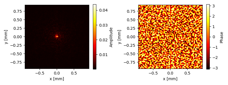
@@ -0,0 +1,23 @@
+import numpy as np
+import sys
+sys.path.insert(0, '/Users/joost/Dropbox/Werk/PhD/Documents/Published/FourierOptics GitHub release/')
+# sys.path.insert(0, '/Users/joost/Dropbox/Werk/PhD/Analyses/Python/Analytical/Fourier Optics')
+from fourierOptics import *
+
+if __name__ == '__main__':
+	# Initiate MICADO paraxial model
+	mcd = ParaxialMICADO()
+	# mcd.plot_ray_trace()
+
+	print(mcd.platescale)
+	# Initiate WFE object
+	wfe = WavefrontError(mcd.n, mcd.m)
+
+	# Generate PSD surfaces
+	psd = wfe.generate_height_map(200e-6, 2, 1)
+
+	# Add it to ADC-P1
+	mcd.ELT_ADC.p1.add_wavefront_error(psd)
+
+	# Generate the PSF and plot it
+	E, x, y = mcd.propagate(l=1.35e-3,surface=-1, zoom=True, show=True) # image_output=[-.4,.4,-.4,.4]

demonstration scripts/thesis_propagation_figures.py

@@ -1,6 +1,7 @@
 import numpy as np
 import sys
-sys.path.insert(0, '/Users/joost/Dropbox/Werk/PhD/Analyses/Python/Analytical/Fourier Optics')
+# sys.path.insert(0, '/Users/joost/Dropbox/Werk/PhD/Analyses/Python/Analytical/Fourier Optics')
+sys.path.insert(0, '/Users/joost/Dropbox/Werk/PhD/Documents/Published/FourierOptics GitHub release/')
 from fourierOptics import *
 import matplotlib.pyplot as plt
 from pdb import set_trace
@@ -18,7 +19,8 @@ if __name__ == '__main__':
 	confList = [ ( 1, [-0.4, 0.4, -0.4, 0.4], 	'02_fourier_ELT-IFP.pdf'),
 				 ( 2, [-50, 50, -50, 50], 		'03_fourier_ELT-COL.pdf'),
 				 ( 4, [-50, 50, -50, 50], 		'04_fourier_ELT-MCD-ADC-P2.pdf'),
-				 (-1, [-1.2, 1.2, -1.2, 1.2], 	'05_fourier_ELT-MCD-DET.pdf')]
+				 # (-1, [-1.2, 1.2, -1.2, 1.2], 	'05_fourier_ELT-MCD-DET.pdf')]
+				 (-1, [-1.2/2.669, 1.2/2.669, -1.2/2.669, 1.2/2.669], 	'05_fourier_ELT-MCD-DET.pdf')]
 
 
 	for i in range(len(confList)):
@@ -26,7 +28,7 @@ if __name__ == '__main__':
 		coordinates = confList[i][1]
 		savename = confList[i][2]
 		E, x, y = mcd.propagate(l=1.35e-3, surface=s, image_output=coordinates,
-								 zoom=False, show=False, save=savename)
+								 zoom=False, show=True, save=False)
 
 	Eout, x, y = mcd.propagate(l=1.35e-3, surface=0, zoom=False, show=False)
 	x /= 1e3 # convert to m
@@ -47,5 +49,5 @@ if __name__ == '__main__':
 	_ax2.set_ylabel('y [m]')
 	_fig.colorbar(_im2, ax=_ax2, label='Phase')
 	plt.tight_layout()
-	plt.savefig('01_fourier_ELT-M1.pdf', bbox_inches='tight', transparent=True)
+	# plt.savefig('01_fourier_ELT-M1.pdf', bbox_inches='tight', transparent=True)
 	plt.close()#show()

fourierOptics/__init__.py

@@ -3,9 +3,9 @@ from .fourier import *
 from .gaussian import *
 from .opticalTrain import *
 from .optics import *
+from .micado import *
 from .profiles import *
 from .psfFitter import *
 from .wavefrontErrors import *
 from .misc import *
-from .micado import *
 from .atmosphere import *

fourierOptics/atmosphere.py

@@ -1,6 +1,8 @@
 import numpy as np
 import scipy.special as spc
 from .misc import *
+import pyfftw
+import os
 
 '''
 	Various functions to simulate a seeing limited PSF. These functions are
@@ -53,6 +55,45 @@ def fried_r0(wvl, seeing):
 	return r0
 
 
+def r0converter(r0, lambda1, lambda2):
+	'''
+		Equivalent to anisocado.psf_utils.r0Converter()
+
+		Converts a r0 defined at some wavelength lambda1,
+		into a r0' at lambda2.
+		Lambda1 and 2 shall be in the SAME unit.
+		Returned r0 will be in the SAME unit than the input one.
+		Example::
+			r0_K = r0Converter(0.12, 500, 2200)
+	'''
+	return r0 * ( lambda2 / lambda1 )**( 6/5.)
+
+
+def r0_at_observed_zenith_distance(r0_at_zenith, zenith_distance):
+	'''
+		The seeing/r0 actually perceived by a telescope depends on the zenith
+		distance. This function converts a r0 given at zenith into the real r0
+		actually observed by the telescope.
+
+		Parameters:
+		-----------
+		r0_at_zenith    - Float or Array
+				Fried length r0 at zenith (degrees) in the wavelength of
+				interest. See also fried_r0() and r0converter().
+		zenith_distance - Float or Array. 
+				Observed zenith distance (degrees)
+
+		Returns:
+		r0 				- Float or Array
+				Observed r0 at the observed zenith distance
+		
+	'''
+	z = zenith_distance * np.pi / 180  # the same, in radians
+	r0 = r0_at_zenith * np.cos(z)**(3./5)
+	return r0
+
+
+
 def airmass(z):
 	'''
 		Converts zenith angle in degrees to airmass
@@ -83,7 +124,7 @@ def spectrum(k, r0, L0=25):
 	return spectrum 
 
 
-def add_seeing(wvl, sng, field_tuple):
+def add_seeing(wvl, sng, field_tuple, focal_length=3200):
 	'''
 		Computes the seeing limited PSF for a supplied amplitude
 		distribution.
@@ -96,6 +137,8 @@ def add_seeing(wvl, sng, field_tuple):
 			Atmospheric seeing in arcseconds.
 		field_tuple - Tuple 
 			Contains the PSF information (amplitude array, x coordinates, y coordinates)
+		focal_length - float
+			Focal length in mm of the telescope used.
 		
 		Returns:
 		psf_seeing 	- Array
@@ -105,8 +148,8 @@ def add_seeing(wvl, sng, field_tuple):
 	r01   = fried_r0(wvl, seeing=sng) * 1e3
 	A_psf, x_psf, y_psf = field_tuple
 	n,m = np.shape(x_psf)
-	fx = x_psf / (3200*wvl)
-	fy = y_psf / (3200*wvl)
+	fx = x_psf / (focal_length*wvl)
+	fy = y_psf / (focal_length*wvl)
 	dk = find_pixel_scale(fx)
 
 	# von-Karman spectrum of the atmosphere for the given frequencies in k-space
@@ -133,3 +176,398 @@ def add_seeing(wvl, sng, field_tuple):
 	return psf_seeing
 
 
+
+
+
+def add_scao(wvl, sng, field_tuple, focal_length=2059940, perfect_scao=False, 
+			dactu=540.3, offx=0, offy=0):
+	'''
+		After adding seeing, we would like to add Adaptive Optics to the system.
+		Based on the 'anisocado' package, I will try to reproduce an AO corrected
+		PSF for MICADO, with a nice seeing halo around it.
+
+		Some of the functions from anisocado will be reused or modified to make it
+		work for me.
+
+		Parameters
+		----------
+		wvl 		-	Float
+			Wavelength in mm corresponding to the supplied PSF
+		sng 		- 	Float
+			Atmospheric seeing in arcseconds.
+		field_tuple - Tuple 
+			Contains the PSF information (amplitude array, x coordinates, y coordinates)
+		focal_length - float
+			Focal length in mm of the telescope used.
+		perfect_scao - bool
+			Whether or not SCAO errors should be considered. If true, time delay,
+			anisoplanatism and others are added.
+		dactu 	- 	float
+			Distance between actuators on the DM in millimeters.
+		offx, offy - float
+			Angular offset in arcseconds from the SCAO guide star relative to the 
+			observed target. This will simulate anisoplanatism.
+		
+		Returns:
+		psf_seeing 	- Array
+			2D array containing the new seeing limited PSF information.
+
+	'''
+	L0 = 25*1e3 # outer scale parameter of the turbulence cells (in mm)
+	rms_wfe_mm = 100. * 1e-6 # Overall system wavefront error
+
+	r01   = fried_r0(wvl, seeing=sng) * 1e3
+	A_psf, x_psf, y_psf = field_tuple
+	n,m = np.shape(x_psf)
+	fx  = x_psf / (focal_length*wvl)
+	fy  = y_psf / (focal_length*wvl)
+	dk  = find_pixel_scale(fx)
+
+
+	# von-Karman spectrum of the atmosphere for the given frequencies in k-space
+	W_atm   = spectrum(np.hypot(fx.real, fy.real), r0=r01, L0=L0)
+	W_atm[int(n/2),int(m/2)] = 0
+
+	# M4 is the ELT deformable mirror that is used for SCAO
+	M4 = define_DM_FrequencyArea(fy, fx, dactu=dactu)
+
+	# [SKIPPED] W_aniso = anisoplanaticSpectrum(Cn2h, layerAltitude, L0, offx, offy, wvl, fx, fy, W_atm, M4)
+
+	# Assuming the correction is perfect within the controlled frequencies
+	W_fit = W_atm.copy()
+	W_fit[M4] = 0.0
+
+	if perfect_scao:
+		# Effect of isoplanatic errors
+		layerAltitude, Cn2h = get_Cn2h()
+		W_aniso = get_anisoplanatic_spectrum(Cn2h, layerAltitude, offx, offy, fx, fy, W_atm, M4)
+		
+		W_combined = W_fit + W_aniso
+
+
+	else:
+		# Alias effects, primarily at the edges of the DM
+		W_alias = get_aliasing_spectrum(fy, fx, r0=r01, L0=L0, M4=M4)
+
+		# Effect of isoplanatic errors
+		layerAltitude, Cn2h = get_Cn2h()
+		W_aniso = get_anisoplanatic_spectrum(Cn2h, layerAltitude, offx, offy, fx, fy, W_atm, M4)
+		
+		# Effect of something...
+		W_bp    = get_Bp_spectrum(fy, fx, W_atm=W_atm, DM=M4)
+		
+		# Effect of overall wavefront error contribution. Static.
+		W_other = get_wfe_spectrum(rms_wfe_mm, M4, dk, wvl)
+		
+		# W_aniso is so much smaller than all the other contributors!
+		W_combined = W_fit + W_aniso + W_alias + W_bp + W_other				   
+
+	# Compute the atmospheric OTF
+	# According to Roddier 1981, the atmospheric OTF can be derived from the phase structure function
+	# assuming that the phase is stationary accross the pupil and behaves as a Gaussian variable
+	# Bphi = np.fft.fft2(np.fft.ifftshift(W_combined))*dk**2
+	Bphi = fftw_forward(np.fft.ifftshift(W_combined))*dk**2
+	Dphi = np.fft.ifftshift((2 * (Bphi[0,0] - Bphi))) # ifftshift in Bphi en Dphi!
+	otf_ao = np.exp(-0.5*Dphi)
+
+	# Compute the OTF of the supplied PSF
+	# We can derive the OTF from the inverse Fourier transform of the PSF
+	psf = np.abs(A_psf)**2
+	otf_psf = np.fft.fftshift(fftw_inverse(np.fft.fftshift(psf)))
+	otf_psf = otf_psf/otf_psf.max()
+
+	# Compute the seeing-limited PSF
+	# Multiplication of OTF and then Fourier transform
+	otf  = otf_psf * otf_ao
+	psf_seeing = np.fft.fftshift(fftw_forward(np.fft.ifftshift(otf)))
+	return psf_seeing
+
+
+def define_DM_FrequencyArea(kx, ky, rotdegree=0, dactu=540.3):
+	'''
+		From anisocado.psf_utils.defineDmFrequencyArea()
+
+		<kx>        : spatial frequency produced by the
+					  function computeSpatialFreqArrays() (metres^-1)
+		<ky>        : idem kx
+		<rotdegree> : rotation of M4 (degrees)
+		<dactu>     : value of actuator pitch of M4 (metres)
+		
+		The function returns the 2D domain of spatial frequencies which can be
+		impacted by M4, i.e. the M4 compensation domain.
+		Underlying assumtions are than M4 is of an hexagonal pattern, with an
+		inter-actuator distance <dactu> set by default to 54.03 cm (=540.3 mm).
+		Result is returned with a frequency corner-centred representation.
+	'''
+
+	# cut-off frequency
+	fc = (1./np.sqrt(3)) / dactu
+
+	# mask frequency definition
+	A = np.pi/3  # 60 degrees
+	A0 = rotdegree * np.pi / 180
+	msk = np.abs(np.cos(A0)*ky+np.sin(A0)*kx)<fc
+	msk = np.logical_and(msk, np.abs(np.cos(A+A0)*ky+np.sin(A+A0)*kx)<fc)
+	msk = np.logical_and(msk, np.abs(np.cos(2*A+A0)*ky+np.sin(2*A+A0)*kx)<fc)
+	k = np.sqrt(kx**2 + ky**2)
+	msk = np.logical_and(msk, k < (fc*1.115))
+	return msk
+
+
+def get_aliasing_spectrum(kx, ky, r0, L0, M4, dssp=0.4015):
+	'''
+		All units scale with millimeter (either in mm^-1 or mm)	
+	'''
+	# convert dssp from meters to millimeters
+	dssp *= 1e3
+	ke = 1.0 / dssp  # computes the sampling spatial-frequency of the WFS
+
+	kxt = kx[M4]
+	kyt = ky[M4]
+	Wt  = ((kxt-ke)**2 + kyt**2 + 1./L0**2.)**(-11./6)
+	Wt += ((kxt+ke)**2 + kyt**2 + 1./L0**2.)**(-11./6)
+	Wt += (kxt**2 + (kyt-ke)**2 + 1./L0**2.)**(-11./6)
+	Wt += (kxt**2 + (kyt+ke)**2 + 1./L0**2.)**(-11./6)
+	Wt *= 0.0228956 * r0**(-5./3)
+	Walias = np.zeros(M4.shape)
+	Walias[M4] = Wt.real
+
+	return Walias
+
+
+def get_anisoplanatic_spectrum(Cn2h, layerAltitude, offx, offy,
+						  kx, ky, atm_psd, DM):
+	'''
+	From anisocado.psf_utils.anisoplanaticSpectrum(), modified to accomodate
+	length in millimeters, i.s.o. meters.
+
+	<Cn2h>          : list of normalised (np.sum(Cn2h)==1.0) strengh of
+					  turbulence of each layer (no unit)
+	<layerAltitude> : list of altitudes of the turbulence layers (metres)
+	<L0>            : value of the outer scale (metres)
+	<offx>          : off-axis distance of the star along X axis (arcsec)
+	<offy>          : idem along Y axis (arcsec)
+	<wavelength>    : wavelength (metres)
+	<kx>            : spatial frequency produced by
+					  the function computeSpatialFreqArrays() (metres^-1)
+	<ky>            : idem kx
+	<atm_psd>      : turbulent spectrum from function computeWiener()
+	<DM>            : frequency domain of M4 (boolean) computed by the
+					  function M4 = defineDmFrequencyArea(kx, ky, 0)
+	Computes the phase spectrum (spatial frequencies) contribution due to the
+	anisoplanatism in the AO compensation for a source located off-axis from
+	the SCAO guide star by some amount (offx, offy).
+	In input, the distribution of the turbulence in altitude is given.
+	Result is returned with a frequency corner-centred representation.
+	'''
+
+	# number of turbulent layers involved in that computation
+	nlayers = len(Cn2h)
+
+	# conversion arcsec to radians
+	RASC = 206264.8062471
+
+	# prepare memory alloc for transfer function of anisoplanatism
+	Haniso = np.zeros(kx.shape)
+
+	# loop over turbulent layers, summing transfer function of each layer
+	for i in range(nlayers):
+		dx = layerAltitude[i] * offx / RASC # shift in millimetres on the layer in X
+		dy = layerAltitude[i] * offy / RASC # idem, in Y
+		tmp = (2j*np.pi*dx)*kx + (2j*np.pi*dy)*ky
+		Haniso += Cn2h[i] * np.abs(1 - np.exp( tmp ))**2
+
+	# now applying the transfer function on the Wiener spectrum, only in the
+	# spatial frequency range of M4
+	Waniso = np.zeros(Haniso.shape)
+	Waniso[DM] = Haniso[DM] * atm_psd[DM]
+
+	return Waniso
+
+
+def get_Bp_spectrum(kx, ky, W_atm, DM, V=10, Fe=500, tret=4e-3, gain=0.3):
+	'''
+		From anisocado.psf_utils.computeBpSpectrum()
+
+		V = 10. 	 - Wind speed in m/s
+		Fe = 500. Hz - response rate
+		tret = 0.004 - time delay in seconds
+		gain = 0.3   - gain of the control loop
+		f = computeBpSpectrum(kx, ky, V, Fe, tret, gain, W, M4)
+	'''
+	k = np.sqrt(kx*kx + ky*ky)
+	nu = k * V / np.sqrt(2)
+	Wbp = hcor(nu, Fe, tret, gain, 500) * W_atm
+	Wbp[np.logical_not(DM)] = 0.
+	return Wbp
+
+
+def hcor(freq, Fe, tret, G, BP, an=True):
+	'''
+	From anisocado.psf_utils.hcor()
+
+	***** Fonction extraite de STYC le 9 Jan 2013 *****
+	The option an=1 sets the integrator to "analog". Doing this, an
+	extra 1/2 frame delay is added compared to case of the numeric
+	integrator an=0.
+	<tret> is the delay expressed as a *time in seconds*, between the
+	end of the integration and the start of the command.
+	'''
+
+	Te = 1. / Fe
+	p = 1j * 2 * np.pi * freq + 1e-12
+
+	Hint = 1./(1-np.exp(-p*Te)) 		# numeric integrator
+	Hccd = (1.-np.exp(-p*Te))/(p*Te)  	# echant bloqueur avec retard 1/2 trame
+	Hdac = Hccd                    		# echant bloqueur avec retard 1/2 trame
+	Hret = np.exp(-p*tret)
+	Hmir = 1./(1. + 1j*freq/BP)
+	Hbo = Hint * Hccd * Hdac * Hret * Hmir
+	Hcor   = 1./abs(1 + Hbo*G)**2
+	return Hcor
+
+
+def get_wfe_spectrum(wfe_rms, M4, uk, wavelength):
+	'''
+		<nmRms>  : number of nm rms
+		<M4>     : frequency domain of M4 (boolean) computed by the
+						  function M4 = defineDmFrequencyArea(kx, ky, 0)
+		<uk> : # size of the 'spatial frequency pixel' in m^-1
+		<wavelength>    : wavelength (metres)
+		Example::
+			N = 512
+			pixelSize = 4.2
+			L0 = 25.0
+			offx, offy = (34., 12.)
+			wavelength = 1.65e-6
+			kx, ky, uk = computeSpatialFreqArrays(N, pixelSize, wavelength)
+			M4 = defineDmFrequencyArea(kx, ky, 0)
+			nmRms = 250.
+			f = otherSpectrum(nmRms, M4, uk, wavelength)
+	'''
+	fact = 2 * np.pi * wfe_rms / uk / wavelength
+	fact = fact**2
+	tot = np.sum(M4)
+	Wothers = np.zeros(M4.shape)
+	Wothers[M4] = fact / tot
+
+	return Wothers
+
+
+
+def get_Cn2h(myProfile='EsoMedian'):
+	'''
+	From anisocado.psf_utils.get_atmospheric_turbulence()
+
+	Returns the relative level of turbulence at a given height
+	Note: The np.sum(Cn2h) = 1.0
+	Turbulence profile have been taken from ESO-258292: "Relevant Atmospheric
+	Parameters for E-ELT AO Analysis and Simulations".
+	The following 3 turbulence profile are currently available:
+	* ``EsoQ1``
+		Best atmospheric conditions - First Quartile Armazones atmospheric
+		turbulence profile
+	* ``EsoMedian`` [also ``officialEsoMedian``]
+		Median atmospheric conditions - Median Armazones atmospheric turbulence
+		profile
+	* ``EsoQ4``
+		Worst atmospheric conditions - First Quartile Armazones atmospheric
+		turbulence profile
+	Additional turbulence profiles include:
+	* ``oldEso``
+		The old ESO profile from before 2010. Cn2h paramateres are taken from
+		ref. E-SPE-ESO-276-0206_atmosphericparameters
+	* ``gendron``
+		The Gendron profile. Short, fast. Saves CPU. Carbon efficient.
+		The np.sum(Cn2h) = 1.0 is hyper-guaranteed here.
+	
+	Parameters
+	----------
+	myProfile : str, optional
+		Profile name: ['EsoQ1', 'EsoMedian', 'EsoQ4', 'oldEso', 'gendron']
+	
+	Returns
+	-------
+	layerAltitude : list of floats
+		[m] height of layer above ground
+	Cn2h : list of floats
+		Relative strength of turbulence
+	'''
+
+	layerAltitude, Cn2h = [], []
+
+	if myProfile == 'oldEso':
+		layerAltitude = [47., 140, 281, 562, 1125, 2250, 4500, 9000, 18000.]
+		Cn2h = [0.5224, 0.026, 0.0444, 0.116, 0.0989,
+				0.0295, 0.0598, 0.043, 0.06]
+
+	elif myProfile == 'officialEsoMedian' or myProfile == 'EsoMedian' :
+		layerAltitude = [30, 90, 150, 200, 245, 300, 390, 600, 1130, 1880, 2630,
+						 3500, 4500, 5500, 6500, 7500, 8500, 9500, 10500, 11500,
+						 12500, 13500, 14500, 15500, 16500, 17500, 18500, 19500,
+						 20500, 21500, 22500, 23500, 24500, 25500, 26500]
+		Cn2h = [24.2, 12, 9.68, 5.9, 4.73, 4.73, 4.73, 4.73, 3.99, 3.24, 1.62,
+				2.6, 1.56, 1.04, 1, 1.2, 0.4, 1.4, 1.3, 0.7, 1.6, 2.59, 1.9,
+				0.99, 0.62, 0.4, 0.25, 0.22, 0.19, 0.14, 0.11, 0.06, 0.09, 0.05,
+				0.04]
+		Cn2h = np.array(Cn2h)
+		Cn2h /= np.sum(Cn2h)
+
+	elif myProfile == 'EsoQ1':
+		layerAltitude = [30, 90, 150, 200, 245, 300, 390, 600, 1130, 1880, 2630,
+						 3500, 4500, 5500, 6500, 7500, 8500, 9500, 10500, 11500,
+						 12500, 13500, 14500, 15500, 16500, 17500, 18500, 19500,
+						 20500, 21500, 22500, 23500, 24500, 25500, 26500]
+		Cn2h = [22.6, 11.2, 10.1, 6.4, 4.15, 4.15, 4.15, 4.15, 3.1, 2.26, 1.13,
+				2.21, 1.33, 0.88, 1.47, 1.77, 0.59, 2.06, 1.92, 1.03, 2.3, 3.75,
+				2.76, 1.43, 0.89, 0.58, 0.36, 0.31, 0.27, 0.2, 0.16, 0.09, 0.12,
+				0.07, 0.06]
+		Cn2h = np.array(Cn2h)
+		Cn2h /= np.sum(Cn2h)
+
+	elif myProfile == 'EsoQ4':
+		layerAltitude = [30, 90, 150, 200, 245, 300, 390, 600, 1130, 1880, 2630,
+						 3500, 4500, 5500, 6500, 7500, 8500, 9500, 10500, 11500,
+						 12500, 13500, 14500, 15500, 16500, 17500, 18500, 19500,
+						 20500, 21500, 22500, 23500, 24500, 25500, 26500]
+		Cn2h = [23.6, 13.1, 9.81, 5.77, 6.58, 6.58, 6.58, 6.58, 5.4, 3.2, 1.6,
+				2.18, 1.31, 0.87, 0.37, 0.45, 0.15, 0.52, 0.49, 0.26, 0.8, 1.29,
+				0.95, 0.49, 0.31, 0.2, 0.12, 0.1, 0.09, 0.07, 0.06, 0.03, 0.05,
+				0.02, 0.02]
+		Cn2h = np.array(Cn2h)
+		Cn2h /= np.sum(Cn2h)
+
+	elif myProfile == 'gendron':
+		Cn2h = [1.0]
+		layerAltitude = [4414.]
+
+	layerAltitude = (np.asarray(layerAltitude) * 1e3).tolist()
+	return layerAltitude, Cn2h
+
+
+def fftw_forward(Ain):
+	# Initialization of input array
+	_A_in 		= pyfftw.empty_aligned(Ain.shape, dtype='complex128')
+	_A_in[:] 	= Ain
+
+	# Initialization of output array
+	_A_out 		= pyfftw.empty_aligned(Ain.shape, dtype='complex128')
+
+	# Invoking Pythors FFTW
+	_FFTW_Obj 	= pyfftw.FFTW( _A_in, _A_out, axes=(0,1), direction='FFTW_FORWARD', threads=os.cpu_count(), flags=('FFTW_ESTIMATE',))
+	_FFTW_Obj()
+	return _A_out
+
+def fftw_inverse(Ain):
+	# Initialization of input array
+	_A_in 		= pyfftw.empty_aligned(Ain.shape, dtype='complex128')
+	_A_in[:] 	= Ain
+
+	# Initialization of output array
+	_A_out 		= pyfftw.empty_aligned(Ain.shape, dtype='complex128')
+
+	# Invoking Pythors FFTW
+	_FFTW_Obj 	= pyfftw.FFTW( _A_in, _A_out, axes=(0,1), direction='FFTW_BACKWARD', threads=os.cpu_count(), flags=('FFTW_ESTIMATE',))
+	_FFTW_Obj()
+	return _A_out
+

fourierOptics/fourier.py

@@ -6,6 +6,7 @@ from scipy.optimize import leastsq
 from matplotlib.ticker import FormatStrFormatter
 from matplotlib.colors import LogNorm
 import pyfftw
+import os
 from .misc import find_pixel_scale
 
 class FourierOptics:
@@ -68,7 +69,7 @@ class FourierOptics:
 		_E_xy0[:] 	= np.fft.ifftshift(A)  					# use ifftshift to shift origin to start array
 		_IntensityNormFactor = np.sum(np.abs(_E_xy0)**2)	# Factor to scale the intensity after the FFTs
 		_Az0 		= pyfftw.empty_aligned((_n,_m), dtype='complex128')
-		_FFTW_Obj 	= pyfftw.FFTW( _E_xy0, _Az0, axes=(0,1), direction='FFTW_BACKWARD', threads=6, flags=('FFTW_ESTIMATE',))
+		_FFTW_Obj 	= pyfftw.FFTW( _E_xy0, _Az0, axes=(0,1), direction='FFTW_BACKWARD', threads=os.cpu_count(), flags=('FFTW_ESTIMATE',))
 		_FFTW_Obj()
 
 		# E-field at z=dz is the fourier transform of A(z=0)*e^(-ikz)
@@ -86,7 +87,7 @@ class FourierOptics:
 		_A_in 		= pyfftw.empty_aligned((_n,_m), dtype='complex128')
 		_A_in[:] 	= _Az0 * _phaseFactor
 
-		_FFTW_Obj2 	= pyfftw.FFTW( _A_in, _E_xyz, axes=(0,1), direction='FFTW_FORWARD', threads=6, flags=('FFTW_ESTIMATE',))
+		_FFTW_Obj2 	= pyfftw.FFTW( _A_in, _E_xyz, axes=(0,1), direction='FFTW_FORWARD', threads=os.cpu_count(), flags=('FFTW_ESTIMATE',))
 		_FFTW_Obj2()
 		_E_xyz 		= np.fft.fftshift(_E_xyz) 				# use fftshift to move the origin from edge to center
 		_E_xyz /= np.sqrt(_IntensityNormFactor) 			# Normalization back to initial energy.
@@ -213,7 +214,7 @@ class FourierOptics:
 		
 		# Output of the FFT evaluated at frequency fx = x / (lambda * z)
 		_U_out 			= pyfftw.empty_aligned((_n,_m), dtype='complex128')
-		_FFTW_Obj		= pyfftw.FFTW( np.fft.ifftshift(_U_in), _U_out, axes=(0,1), direction='FFTW_FORWARD', threads=6, flags=('FFTW_ESTIMATE',))
+		_FFTW_Obj		= pyfftw.FFTW( np.fft.ifftshift(_U_in), _U_out, axes=(0,1), direction='FFTW_FORWARD', threads=os.cpu_count(), flags=('FFTW_ESTIMATE',))
 		_FFTW_Obj()
 		_U_out 			= np.fft.fftshift(_U_out)
 
@@ -365,7 +366,7 @@ class FourierOptics:
 		
 		# Output of the FFT
 		_A_out 			= pyfftw.empty_aligned(PSF.shape, dtype='complex128')
-		_FFTW_Obj		= pyfftw.FFTW( np.fft.ifftshift(_A_in), _A_out, axes=(0,1), direction='FFTW_FORWARD', threads=6, flags=('FFTW_ESTIMATE',))
+		_FFTW_Obj		= pyfftw.FFTW( np.fft.ifftshift(_A_in), _A_out, axes=(0,1), direction='FFTW_FORWARD', threads=os.cpu_count(), flags=('FFTW_ESTIMATE',))
 		_FFTW_Obj()
 		_A_out 			= np.fft.fftshift(_A_out)
 

fourierOptics/micado.py

@@ -9,7 +9,16 @@ from .wavefrontErrors import *
 from .misc import *
 
 
+'''
+Changelog:
 
+Changes w.r.t. the old MICADO paraxial model:
+- Changed focal length of collimator lens from 4278.32701 to 1601.688 mm
+- Changed distance from ADC to collimator lens from 50 mm to 74 mm.
+- Changed thickness of ADC prisms from 25 to 15 mm
+- Changed working F-number (WFNO) from 53.4466 to 20.0269
+- This results in a change of the plate scale from 0.1001 arcsec/mm to 0.2672 arcsec/mm
+'''
 
 class ParaxialMICADO:
 	def __init__(self, l=1.35e-3, n=1001, m=1001, dpix=160, entrance_pupil='ELT'):
@@ -32,7 +41,7 @@ class ParaxialMICADO:
 		self.ELT_FP			= OpticalSurface(name='MCD-IFP')
 		self.ELT_COL		= ParaxialLens(CA=154.54, f=1418.94, name='MCD-COL')
 		self.ELT_ADC 		= ADCObject()
-		self.ELT_CAM		= ParaxialLens(CA=89.2, f=4278.32701, name='MCD-CAM')
+		self.ELT_CAM		= ParaxialLens(CA=89.2, f=1601.688, name='MCD-CAM')
 		self.ELT_DET		= OpticalSurface(name='MCD-DET')
 
 		# Built optical train
@@ -41,11 +50,12 @@ class ParaxialMICADO:
 		self.MCD.add_object(self.ELT_FP, 		dist=self.ELT_MIRROR.f)
 		self.MCD.add_object(self.ELT_COL, 		dist=self.ELT_COL.f)
 		self.ELT_ADC.add_to_optical_train(self.MCD, 1209.4718)
-		self.MCD.add_object(self.ELT_CAM, 		dist=50)
+		self.MCD.add_object(self.ELT_CAM, 		dist=74)
 		self.MCD.add_object(self.ELT_DET, 		dist=self.ELT_CAM.f)
 
 		self.last_PSF 		= None
 		self.clean_PSF 		= None
+		self.pixelscale 	= 4e-3 # arcseconds/pixel
 		self.platescale 	= self.set_plate_scale()
 		print ('Your resolution is {}x{} with a pixel size of {}'.format(self.n,self.m,self.dpix))
 		print('This means your grid is {} mm by {} mm, with each pixel {} mm.'.format(
@@ -233,6 +243,8 @@ class ParaxialMICADO:
 			elif surfaces[s] == self.ELT_FP:
 				if print_progress: print('Propagating from ELT-IFP to MCD-COL')
 				Ein = Eout
+				if self.ELT_FP.wavefrontError:
+					Ein *= self.ELT_FP.phase_delay(x, y, l, ip_type='phase')
 				Eout, x, y = fou.fresnel_propagation(Ein, x, y, dz=self.ELT_COL.f, oversample=None, 
 					show=show[s], save=saveList[s], outputCoordinates=output_coordinates[s], 
 					apply_interpolation=apply_ip[s], tx=tilt_x[s], ty=tilt_y[s])
@@ -332,7 +344,7 @@ class ParaxialMICADO:
 								[-120, 120, -120, 120],
 								[-120, 120, -120, 120],
 								[-120, 120, -120, 120],
-								[-2.5, 2.5, -2.5, 2.5]
+								[-2.5/2.669, 2.5/2.669, -2.5/2.669, 2.5/2.669]
 							  ]
 		elif coordinates is not None:
 			_coordinatesList = coordinates
@@ -384,12 +396,12 @@ class ParaxialMICADO:
 			_apply_ip[surf] = True
 		return _apply_ip
 
-	def set_plate_scale(self):
+	def set_plate_scale(self, wfno=20.0269):
 		'''
 			Returns the platescale of this paraxial MICADO
 			model in arcseconds/mm.
 		'''
-		_ps = (3600*180/np.pi) / (self.ELT_MIRROR.CA * 53.4466)
+		_ps = (3600*180/np.pi) / (self.ELT_MIRROR.CA * wfno)
 		self.platescale = _ps
 		return _ps
 
@@ -522,7 +534,7 @@ class ParaxialMICADO:
 										a2y=np.deg2rad(self.ELT_ADC.p4.tilt2y),
 										n_glass=self.ELT_ADC.p4.find_refractive_index(self.l, unit='millimeter'))
 		positions_and_angles.append([xp,yp,np.degrees(tx),np.degrees(ty)])
-		xp, yp, tx,ty = get_free_space_propagation_rtm(xp,yp,tx,ty,50)
+		xp, yp, tx,ty = get_free_space_propagation_rtm(xp,yp,tx,ty,74)
 
 		# ELT-MCD-CAM:
 		xp, yp, tx, ty = get_paraxial_lens_rtm(xp, yp, tx, ty, self.ELT_CAM.f, self.ELT_CAM.f)
@@ -546,8 +558,8 @@ class ParaxialMICADO:
 							6.84022e5+1418.94+1209.4718 + 15 + 1 + 15 + 8 + 15, # ADC p3
 							6.84022e5+1418.94+1209.4718 + 15 + 1 + 15 + 8 + 15 + 1, # Between p3 and p4
 							6.84022e5+1418.94+1209.4718 + 15 + 1 + 15 + 8 + 15 + 1 + 15, # ADC p4
-							6.84022e5+1418.94+1209.4718 + 15 + 1 + 15 + 8 + 15 + 1 + 15 + 50, # MCD-CAM
-							6.84022e5+1418.94+1209.4718 + 15 + 1 + 15 + 8 + 15 + 1 + 15 + 50 + 4278.32701 # Focal plane
+							6.84022e5+1418.94+1209.4718 + 15 + 1 + 15 + 8 + 15 + 1 + 15 + 74, # MCD-CAM
+							6.84022e5+1418.94+1209.4718 + 15 + 1 + 15 + 8 + 15 + 1 + 15 + 74 + 1601.688 # Focal plane
 							])
 		return x_out, y_out, tx_out, ty_out, z_out
 
@@ -640,7 +652,7 @@ class ParaxialMICADO:
 		# Fourth prism
 		xp, yp, tx,ty = get_free_space_propagation_rtm(xp,yp,tx,ty,self.ELT_ADC.p4.thickness)
 		positions_and_angles.append([xp,yp,np.degrees(tx),np.degrees(ty)])
-		xp, yp, tx,ty = get_free_space_propagation_rtm(xp,yp,tx,ty,50)
+		xp, yp, tx,ty = get_free_space_propagation_rtm(xp,yp,tx,ty,74)
 
 		# ELT-MCD-CAM:
 		xp, yp, tx, ty = get_paraxial_lens_rtm(xp, yp, tx, ty, self.ELT_CAM.f, self.ELT_CAM.f)
@@ -664,8 +676,8 @@ class ParaxialMICADO:
 							6.84022e5+1418.94+1209.4718 + 15 + 1 + 15 + 8 + 15, # ADC p3
 							6.84022e5+1418.94+1209.4718 + 15 + 1 + 15 + 8 + 15 + 1, # Between p3 and p4
 							6.84022e5+1418.94+1209.4718 + 15 + 1 + 15 + 8 + 15 + 1 + 15, # ADC p4
-							6.84022e5+1418.94+1209.4718 + 15 + 1 + 15 + 8 + 15 + 1 + 15 + 50, # MCD-CAM
-							6.84022e5+1418.94+1209.4718 + 15 + 1 + 15 + 8 + 15 + 1 + 15 + 50 + 4278.32701 # Focal plane
+							6.84022e5+1418.94+1209.4718 + 15 + 1 + 15 + 8 + 15 + 1 + 15 + 74, # MCD-CAM
+							6.84022e5+1418.94+1209.4718 + 15 + 1 + 15 + 8 + 15 + 1 + 15 + 74 + 1601.688 # Focal plane
 							])
 		return x_out, y_out, tx_out, ty_out, z_out
 

fourierOptics/micado_old.py

@@ -0,0 +1,798 @@
+import numpy as np
+from .fourier import *
+from .gaussian import *
+from .opticalTrain import *
+from .optics import *
+from .profiles import *
+from .psfFitter import *
+from .wavefrontErrors import *
+from .misc import *
+
+
+
+
+class ParaxialMICADO:
+	def __init__(self, l=1.35e-3, n=1001, m=1001, dpix=160, entrance_pupil='ELT'):
+		self.l 				= l
+		self.dpix 			= dpix
+		self.n, self.m 		= n, m
+		self.x, self.y 		= np.meshgrid(np.linspace(-n/2*dpix, n/2*dpix, n), np.linspace(-m/2*dpix, m/2*dpix, m))	
+		if entrance_pupil == 'ELT':
+			self.ELT_MASK 		= Profiles().ELT_pupil(n,m,dpix).astype('complex128')
+		elif entrance_pupil == 'obscured':
+			r1 = 38542/2
+			r2 = 10700/2
+			self.ELT_MASK 		= Profiles().obscured_top_hat(r1, r2, n, m, dpix).astype('complex128')
+		elif entrance_pupil == 'open':
+			r1 = 38542/2
+			self.ELT_MASK 		= Profiles().top_hat(r1, n, m, dpix).astype('complex128')
+
+		# Built optical system elements
+		self.ELT_MIRROR 	= ParabolicMirror(dx=0, dy=0, name='ELT-paraxial', CA=38542, f=6.84022e5)	
+		self.ELT_FP			= OpticalSurface(name='MCD-IFP')
+		self.ELT_COL		= ParaxialLens(CA=154.54, f=1418.94, name='MCD-COL')
+		self.ELT_ADC 		= ADCObject()
+		self.ELT_CAM		= ParaxialLens(CA=89.2, f=4278.32701, name='MCD-CAM')
+		self.ELT_DET		= OpticalSurface(name='MCD-DET')
+
+		# Built optical train
+		self.MCD 			= OpticalTrain()
+		self.MCD.add_object(self.ELT_MIRROR, 	dist=0)
+		self.MCD.add_object(self.ELT_FP, 		dist=self.ELT_MIRROR.f)
+		self.MCD.add_object(self.ELT_COL, 		dist=self.ELT_COL.f)
+		self.ELT_ADC.add_to_optical_train(self.MCD, 1209.4718)
+		self.MCD.add_object(self.ELT_CAM, 		dist=50)
+		self.MCD.add_object(self.ELT_DET, 		dist=self.ELT_CAM.f)
+
+		self.last_PSF 		= None
+		self.clean_PSF 		= None
+		self.pixelscale 	= 4e-3 # arcseconds/pixel
+		self.platescale 	= self.set_plate_scale()
+		print ('Your resolution is {}x{} with a pixel size of {}'.format(self.n,self.m,self.dpix))
+		print('This means your grid is {} mm by {} mm, with each pixel {} mm.'.format(
+			self.x.max()-self.x.min(), self.y.max()-self.y.min(), self.dpix))
+
+
+	def apply_mask(self, mask, replace=True):
+		'''
+			Set a mask to the ELT entrance pupil.
+		'''
+		if replace:
+			self.ELT_MASK = mask.astype('complex128')
+		elif not replace:
+			self.ELT_MASK *= mask
+
+
+	def set_PSF(self, PSF, x, y, perfect=True):
+		'''
+			If calculating another PSF takes to long,
+			one can set a custom PSF using this 
+			function.
+
+			Can be set as the 'clean' PSF or as another
+			'last' PSF, with the perfect flag.
+		'''
+		if perfect:
+			self.clean_PSF = (PSF, x, y)
+		elif not perfect:
+			self.last_PSF  = (PSF, x, y)
+
+
+	def centroid_shift(self, method='Coupling', reference_PSF=None, **kwargs):
+		'''
+			Do a centroid shift calculation for the given method.
+			This is a quick way of doing it. It only returns the 
+			centroid shift (and uncertainties) and no other parameters.
+		'''
+		assert (self.last_PSF is not None), 'PSF necessary for fitting.'
+		if 'initialGuess' in kwargs:
+			guess_value = kwargs.get('initialGuess')
+
+		if reference_PSF is None:
+			PSF, x, y = self.last_PSF
+		elif reference_PSF is not None:
+			PSF, x, y = reference_PSF
+		fitter = PSFFitter(x.real,y.real,np.abs(PSF)**2)
+
+		if method == 'Coupling':
+			assert (self.clean_PSF is not None), 'Perfect PSF necessary for comparison.'
+			Eclean, xclean, yclean = self.clean_PSF
+			fitted_PSF, popt, var, coupling = fitter.fit_custom_field(Eclean, PSF, return_coupling=True, **kwargs)
+			x0, y0 		= np.asarray(popt).T
+			sx0, sy0 	= np.asarray(np.sqrt(var)).T
+			return x0, y0, sx0, sy0, coupling
+
+		elif method == 'Airy':
+			if 'initialGuess' not in kwargs:
+				guess_value = (0.03**2, 0.0, 0.0, 0.0, 0.03)
+			fitted_PSF, popt, pcov = fitter.fit_airy_PSF(initialGuess=guess_value)
+			_, x0, y0, _, _ = popt
+			pcov_list = [ np.sqrt(pcov[i][i]) for i in range(len(pcov)) ]
+			_, sx0, sy0, _, _ = np.asarray(pcov_list).T
+
+		elif method == 'Obscured Airy':
+			if 'initialGuess' not in kwargs:
+				guess_value = (0.03**2, 0.0, 0.0, 0.0, 0.03)
+			fitted_PSF, popt, pcov = fitter.fit_fixed_obscuration_airy_PSF(initialGuess=guess_value)
+			_, x0, y0, _, _ = popt
+			pcov_list = [ np.sqrt(pcov[i][i]) for i in range(len(pcov)) ]
+			_, sx0, sy0, _, _ = np.asarray(pcov_list).T
+
+		elif method == 'Gaussian':
+			if 'initialGuess' not in kwargs:
+				guess_value = (0.04, 0, 0, 0.01, 0.01, 0, 0)
+			fitted_PSF, popt, pcov = fitter.fit_gaussian_PSF(initialGuess=guess_value)
+			_, x0, y0, _, _, _, _ = popt
+			pcov_list = [ np.sqrt(pcov[i][i]) for i in range(len(pcov)) ]
+			_, sx0, sy0, _, _, _, _ = np.asarray(pcov_list).T
+
+		elif method == 'Moffat':
+			if 'initialGuess' not in kwargs:
+				guess_value = (0.04, 0, 0, 0.01, 0.01, 0, 0, 4)
+			fitted_PSF, popt, pcov = fitter.fit_moffat_PSF(initialGuess=guess_value)
+			_, x0, y0, _, _, _, _, _ = popt
+			pcov_list = [ np.sqrt(pcov[i][i]) for i in range(len(pcov)) ]
+			_, sx0, sy0, _, _, _, _, _ = np.asarray(pcov_list).T
+
+		elif method == 'Barycenter':
+			x0, y0, sx0, sy0 = fitter.fit_barycenter(amplitude=False)
+
+		return x0, y0, sx0, sy0
+
+
+	def propagate(self, l=None, surface=-1, zoom=False, hx=0, hy=0, load_up_to_adc=None, 
+		coordinates=None, show=False, image_output=None, save=None, apply_interpolation=True, 
+		print_progress=True, defocus=None):
+		'''
+			Propagate the input wavefront through the MICADO paraxial
+			model. Optionally the propagation starts at the ADC, if 
+			a data file with the wavefront at that point is defined.
+
+			Parameters:
+			l 				- Desired wavelength of the propagation
+			surface 		- Surface to propagate to. Default: -1 = Detector plane
+			zoom 			- Zoom in on the PSF on the detector?
+			load_up_to_adc 	- Use a .pkl file to load in the wavefront just before the adc.
+			coordinates 	- User defined coordinates that define the propagation sampling.
+			show_final 		- Plots the final amplitude and phase if True.
+
+			Returns:
+			Exyz 			- Complex field with shape n,m describing the amplitude and phase
+							  of the wavefront at the output surface.
+			x, y 			- Corresponding x and y coordinates, in mm.
+		'''
+		# Set up wavelength
+		l = self.l if not l else l
+	
+		# Setting up the arguments for each surface propgation
+		surfaces 			= self.get_surfaces()
+		surface 			= len(surfaces)-1 if surface == -1 else surface
+		coordinatesList 	= self.get_coordinates(coordinates)
+		show,show_final_zoom= self.get_show_image(show, zoom, len(surfaces), surface)
+		output_coordinates 	= self.get_image_coordinates(image_output, coordinatesList, len(surfaces), surface)
+		saveList 			= self.get_save_image(save, len(surfaces), surface)
+		apply_ip 			= self.get_image_interpolation(apply_interpolation, zoom, len(surfaces), surface)
+		tilt_x, tilt_y		= self.get_tilt_angles(hx, hy)
+
+		# Set up the FourierOptics object for propagation
+		fou = FourierOptics(l=l)
+		x, y = self.x, self.y
+		p = 1 # Used as counter for the ADC prisms.
+		
+		# Load the data up to the ADC (useful for many iterations on the same 
+		# calculation, where differences only appear at or after the ADC)
+		if load_up_to_adc is not None:
+			Eout, x, y = load_variable(load_up_to_adc)
+			x = x.real
+			y = y.real
+			s = 4
+		elif load_up_to_adc is None:
+			s = 0
+
+		# Start propgation
+		if print_progress: print('Starting propagation...')
+		while s <= surface:
+			if (surfaces[s] == self.ELT_MASK).all():
+				Ein  = surfaces[s]
+				Eout = surfaces[s]
+				if show[s] or saveList[s]:
+					_fig = plt.figure(figsize=(8,3))
+					_ax = _fig.add_subplot(121)
+					_im = _ax.imshow(np.abs(Eout), cmap='hot', extent=[x.min(), x.max(), y.min(), y.max()])
+					_ax.set_xlim([x.min(), x.max()])
+					_ax.set_ylim([y.min(), y.max()])
+					_ax.set_xlabel('x [mm]')
+					_ax.set_ylabel('y [mm]')
+					_fig.colorbar(_im, ax=_ax, label='Amplitude')
+					_ax2 = _fig.add_subplot(122)
+					_im2 = _ax2.imshow(np.angle(Eout), cmap='hot', extent=[x.min(), x.max(), y.min(), y.max()])
+					_ax2.set_xlim([x.min(), x.max()])
+					_ax2.set_ylim([y.min(), y.max()])
+					_ax2.set_xlabel('x [mm]')
+					_ax2.set_ylabel('y [mm]')
+					_fig.colorbar(_im2, ax=_ax2, label='Phase')
+					plt.tight_layout()
+					if saveList[s]:	
+						plt.savefig(saveList[s], bbox_inches='tight', transparent=True)
+					if show[s]:
+						plt.show()
+					else:
+						plt.close()
+
+			
+			elif surfaces[s] == self.ELT_MIRROR:
+				if print_progress: print('Propagating from ELT-M1 to ELT-IFP')
+				Ein = Eout * self.ELT_MIRROR.phase_delay(x,y,l,paraxial=True)
+				if s == surface and zoom:
+					xzoom, yzoom = x, y
+					Einzoom = Ein
+					fzoom = self.ELT_MIRROR.f
+				Eout, x, y = fou.fresnel_propagation(Ein, x, y, dz=self.ELT_MIRROR.f, oversample=None, 
+					show=show[s], save=saveList[s], outputCoordinates=output_coordinates[s], 
+					apply_interpolation=apply_ip[s], tx=tilt_x[s], ty=tilt_y[s])
+
+			elif surfaces[s] == self.ELT_FP:
+				if print_progress: print('Propagating from ELT-IFP to MCD-COL')
+				Ein = Eout
+				Eout, x, y = fou.fresnel_propagation(Ein, x, y, dz=self.ELT_COL.f, oversample=None, 
+					show=show[s], save=saveList[s], outputCoordinates=output_coordinates[s], 
+					apply_interpolation=apply_ip[s], tx=tilt_x[s], ty=tilt_y[s])
+
+			elif surfaces[s] == self.ELT_COL:
+				if print_progress: print('Propagating from MCD-COL to MCD-ADC-P1')
+				x = x.real
+				y = y.real
+				Ein = Eout * self.ELT_COL.phase_delay(x,y,l, paraxial=True)
+				Eout, x, y = fou.plane_wave_propagation(Ein, x, y, dz=self.MCD.sequentialDistance[3], oversample=None,
+					show=show[s], save=saveList[s], outputCoordinates=output_coordinates[s], tx=tilt_x[s], ty=tilt_y[s])
+
+			elif surfaces[s] == self.ELT_ADC and p == 1:
+				if print_progress: print('Propagating from MCD-ADC-P1 to MCD-ADC-P2')
+				Ein = Eout * self.ELT_ADC.get_phase_delay(x,y,l, theta=None, paraxial=True, prism=1)
+				Eout, x, y = fou.plane_wave_propagation(Ein, x, y, dz=self.MCD.sequentialDistance[4], oversample=None,
+					show=show[s], save=saveList[s], outputCoordinates=output_coordinates[s], tx=tilt_x[s], ty=tilt_y[s])	
+				p += 1
+
+			elif surfaces[s] == self.ELT_ADC and p == 2:
+				if print_progress: print('Propagating from MCD-ADC-P2 to MCD-ADC-P3')
+				Ein = Eout * self.ELT_ADC.get_phase_delay(x,y,l, theta=None, paraxial=True, prism=2)
+				Eout, x, y = fou.plane_wave_propagation(Ein, x, y, dz=self.MCD.sequentialDistance[5], oversample=None,
+					show=show[s], save=saveList[s], outputCoordinates=output_coordinates[s], tx=tilt_x[s], ty=tilt_y[s])	
+				p += 1
+
+			elif surfaces[s] == self.ELT_ADC and p == 3:
+				if print_progress: print('Propagating from MCD-ADC-P3 to MCD-ADC-P4')
+				Ein = Eout * self.ELT_ADC.get_phase_delay(x,y,l, theta=None, paraxial=True, prism=3)
+				Eout, x, y = fou.plane_wave_propagation(Ein, x, y, dz=self.MCD.sequentialDistance[6], oversample=None,
+					show=show[s], save=saveList[s], outputCoordinates=output_coordinates[s], tx=tilt_x[s], ty=tilt_y[s])	
+				p += 1
+
+			elif surfaces[s] == self.ELT_ADC and p == 4:
+				if print_progress: print('Propagating from MCD-ADC-P4 to MCD-CAM')
+				Ein = Eout * self.ELT_ADC.get_phase_delay(x,y,l, theta=None, paraxial=True, prism=4)
+				Eout, x, y = fou.plane_wave_propagation(Ein, x, y, dz=self.MCD.sequentialDistance[7], oversample=None,
+					show=show[s], save=saveList[s], outputCoordinates=output_coordinates[s], tx=tilt_x[s], ty=tilt_y[s])	
+				p += 1
+
+			elif surfaces[s] == self.ELT_DET:
+				if print_progress: print('Propagating from MCD-CAM to MCD-DET')
+				Ein = Eout * self.ELT_CAM.phase_delay(x,y,l, paraxial=True)
+				if defocus is None:
+					defocus = 0
+				if s == surface and zoom:
+					xzoom, yzoom = x.real, y.real
+					Einzoom = Ein
+					fzoom = self.ELT_CAM.f + defocus
+				Eout, x, y = fou.fresnel_propagation(Ein, x, y, dz=self.ELT_CAM.f+defocus, oversample=None, 
+				show=show[s], save=saveList[s], outputCoordinates=output_coordinates[s], 
+				apply_interpolation=apply_ip[s], tx=tilt_x[s], ty=tilt_y[s])
+			s += 1
+
+		if zoom:
+			if print_progress: print('Zooming in on the PSF location...')
+			imax_1, imax_2 = find_maximum(np.abs(Eout))
+			xmax = x[imax_1, imax_2]
+			ymax = y[imax_1, imax_2]
+			ind = s-3 if (s-3)>0 else 0
+			newCoordinates = np.asarray(coordinatesList[ind]) + np.array([xmax, xmax, ymax, ymax])
+			newCoordinates = newCoordinates.real.tolist()
+			Eout, x, y = fou.fresnel_propagation(Einzoom, xzoom, yzoom, dz=fzoom, oversample=None, 
+				show=show_final_zoom, save=saveList[s-1], outputCoordinates=newCoordinates, 
+				apply_interpolation=True, interpol_type='linear', tx=tilt_x[s-1], ty=tilt_y[s-1])
+		
+		if print_progress: print('Propagation finished!')
+		self.last_PSF = (Eout, x, y)
+		return Eout, x, y
+
+
+
+	def get_surfaces(self):
+		_surfaces = [	
+					self.ELT_MASK, 
+					self.ELT_MIRROR,
+					self.ELT_FP, 
+					self.ELT_COL, 
+					self.ELT_ADC,
+					self.ELT_ADC,
+					self.ELT_ADC,
+					self.ELT_ADC,
+					self.ELT_CAM,
+					self.ELT_DET
+					]
+		return _surfaces
+
+
+	def get_coordinates(self, coordinates):
+		# Output coordinates:
+		if coordinates is None:
+			_coordinatesList = [
+								[-1.0, 1.0, -1.0, 1.0],
+								[-200, 200, -200, 200],
+								[-120, 120, -120, 120],
+								[-120, 120, -120, 120],
+								[-120, 120, -120, 120],
+								[-120, 120, -120, 120],
+								[-120, 120, -120, 120],
+								[-2.5, 2.5, -2.5, 2.5]
+							  ]
+		elif coordinates is not None:
+			_coordinatesList = coordinates
+		return _coordinatesList
+
+	def get_show_image(self, show, zoom, N, surf):
+		# Set show values. Will only show the image plane.
+		_showlist = [False] * N
+		_showlist[surf] = show
+		_show_final_zoom = False
+		if zoom:
+			_show_final_zoom = show
+			_showlist[surf] = False
+		_show = _showlist
+		return _show, _show_final_zoom
+
+	def get_image_coordinates(self, image_output, coordinates, N, surf):
+		# Set the image coordinates
+		_output_coordinates = [None] * N
+		_output_coordinates[2] = coordinates[1]
+		if image_output is not None:
+			_output_coordinates[surf] = image_output
+		return _output_coordinates
+
+	def get_save_image(self, save, N, surf):
+		# Set the save values
+		_savelist = [False] * N
+		if save == 'all':
+			_savelist = [
+						'01_ELT_MASK_output.png',
+						'02_ELT_FP_output.png',
+						'03_ELT_MCD_COL_output.png',
+						'04_ELT_MCD_ADC_P1_output.png',
+						'05_ELT_MCD_ADC_P2_output.png',
+						'06_ELT_MCD_ADC_P3_output.png',
+						'07_ELT_MCD_ADC_P4_output.png',
+						'08_ELT_MCD_CAM_output.png',
+						'09_ELT_MCD_DET_output.png',
+						'10_ELT_MCD_DET_output_zoomed.png'
+						]
+		elif save is not None:
+			_savelist[surf] = save
+		return _savelist
+
+	def get_image_interpolation(self, apply_interpolation, zoom, N, surf):
+		# Apply interpolation to the output?
+		_apply_ip = [False] * N
+		if not zoom and apply_interpolation and surf!=2:
+			_apply_ip[surf] = True
+		return _apply_ip
+
+	def set_plate_scale(self):
+		'''
+			Returns the platescale of this paraxial MICADO
+			model in arcseconds/mm.
+		'''
+		_ps = (3600*180/np.pi) / (self.ELT_MIRROR.CA * 53.4466)
+		self.platescale = _ps
+		return _ps
+
+	def get_field_angle(self,hx,hy):
+		fx = hx * 0.0075
+		fy = hy * 0.0075
+		return fx, fy
+
+	def get_tilt_angles(self, hx, hy):
+		'''
+			Returns the propagation angles at each surface
+			in degrees. E.g. near the ADC for hx=1, tx=3.61
+			degrees.
+		'''
+		_x,_y,_tx,_ty,_z = self.perform_ray_trace_without_adc(hx,hy,0,0)
+		_tx[0] = _tx[1]
+		_ty[0] = _ty[1]
+		tx = np.asarray([_tx[i] for i in [0,1,2,3,5,7,9,11,12,13,13]]).flatten()
+		ty = np.asarray([_ty[i] for i in [0,1,2,3,5,7,9,11,12,13,13]]).flatten()
+		return tx, ty
+
+
+	def perform_ray_trace(self,hx,hy,px,py):
+		'''
+			Ray trace the paraxial model of ELT-MICADO
+
+			Parameters
+			----------
+			hx,hy - float or array
+				Normalized field angles
+			px,py - float or array
+				Normalized pupil angles
+
+			Returns
+			-------
+			xout - float or array
+				x-coordinates on all surfaces
+			yout - float or array
+				y-coordinates on all surfaces
+			zout
+				z-coordinates of all surfaces
+
+		'''
+		xout = []
+		yout = []
+
+		# Show simplified 2D ray trace model
+		if type(px)==int or type(px)==float:
+			px = np.array([px])
+		if type(py)==int or type(py)==float:
+			py = np.array([py])
+		if type(hx)==int or type(hx)==float:
+			hx = np.array([hx])
+		if type(hy)==int or type(hy)==float:
+			hy = np.array([hy])
+
+		xp0 = np.asarray(px) * self.ELT_MIRROR.CA/2
+		yp0 = np.asarray(py) * self.ELT_MIRROR.CA/2
+
+		# for xp in range(len(xp0)):
+		positions_and_angles = []
+
+		# Calculate the field angles
+		txin, tyin = self.get_field_angle(hx, hy)
+		txin = np.deg2rad(txin)
+		tyin = np.deg2rad(tyin)
+
+		#Start of system (perhaps at ELT_MASK?)
+		xp, yp, tx, ty = xp0, yp0, txin, tyin
+		positions_and_angles.append([xp,yp,np.degrees(tx),np.degrees(ty)]) # Mask
+
+		# ELT M1
+		xp, yp, tx, ty = get_paraxial_lens_rtm(xp, yp, tx, ty, self.ELT_MIRROR.f, self.ELT_MIRROR.f)
+		positions_and_angles.append([xp,yp,np.degrees(tx),np.degrees(ty)]) # ELT M1
+		xp, yp, tx, ty = get_free_space_propagation_rtm(xp, yp, tx, ty, self.ELT_MIRROR.f)
+
+		# ELT-FP
+		positions_and_angles.append([xp,yp,np.degrees(tx),np.degrees(ty)]) # ELT FP
+		xp, yp, tx, ty = get_free_space_propagation_rtm(xp, yp, tx, ty, self.ELT_COL.f)
+		
+		# ELT-MCD-COL
+		xp, yp, tx, ty = get_paraxial_lens_rtm(xp, yp, tx, ty, self.ELT_COL.f, self.ELT_COL.f)
+		positions_and_angles.append([xp,yp,np.degrees(tx),np.degrees(ty)]) # ELT MCD COL
+		xp, yp, tx, ty = get_free_space_propagation_rtm(xp, yp, tx, ty, 1209.4718)
+
+		# ELT-MCD-ADC
+		# First prism:
+		positions_and_angles.append([xp,yp,np.degrees(tx),np.degrees(ty)])
+		xp, yp, tx, ty = get_prism_rtm( xp,yp,tx,ty,
+										thickness=self.ELT_ADC.p1.thickness,
+										a1x=np.deg2rad(self.ELT_ADC.p1.tilt1x),
+										a2x=np.deg2rad(self.ELT_ADC.p1.tilt2x),
+										a1y=np.deg2rad(self.ELT_ADC.p1.tilt1y),
+										a2y=np.deg2rad(self.ELT_ADC.p1.tilt2y),
+										n_glass=self.ELT_ADC.p1.find_refractive_index(self.l, unit='millimeter'))
+		positions_and_angles.append([xp,yp,np.degrees(tx),np.degrees(ty)])
+		xp, yp, tx,ty = get_free_space_propagation_rtm(xp,yp,tx,ty,1)
+		positions_and_angles.append([xp,yp,np.degrees(tx),np.degrees(ty)])
+
+		# Second prism:
+		xp, yp, tx,ty = get_prism_rtm(	xp,yp,tx,ty,
+										thickness=self.ELT_ADC.p2.thickness,
+										a1x=np.deg2rad(self.ELT_ADC.p2.tilt1x),
+										a2x=np.deg2rad(self.ELT_ADC.p2.tilt2x),
+										a1y=np.deg2rad(self.ELT_ADC.p2.tilt1y),
+										a2y=np.deg2rad(self.ELT_ADC.p2.tilt2y),
+										n_glass=self.ELT_ADC.p2.find_refractive_index(self.l, unit='millimeter'))
+		positions_and_angles.append([xp,yp,np.degrees(tx),np.degrees(ty)])
+		xp, yp, tx,ty = get_free_space_propagation_rtm(xp,yp,tx,ty,8)
+		positions_and_angles.append([xp,yp,np.degrees(tx),np.degrees(ty)])
+
+		# Third prism
+		xp, yp, tx,ty = get_prism_rtm(	xp,yp,tx,ty,
+										thickness=self.ELT_ADC.p3.thickness,
+										a1x=np.deg2rad(self.ELT_ADC.p3.tilt1x),
+										a2x=np.deg2rad(self.ELT_ADC.p3.tilt2x),
+										a1y=np.deg2rad(self.ELT_ADC.p3.tilt1y),
+										a2y=np.deg2rad(self.ELT_ADC.p3.tilt2y),
+										n_glass=self.ELT_ADC.p3.find_refractive_index(self.l, unit='millimeter'))
+		positions_and_angles.append([xp,yp,np.degrees(tx),np.degrees(ty)])
+		xp, yp, tx,ty = get_free_space_propagation_rtm(xp,yp,tx,ty,1)
+		positions_and_angles.append([xp,yp,np.degrees(tx),np.degrees(ty)])
+
+		# Fourth prism
+		xp, yp, tx,ty = get_prism_rtm(  xp,yp,tx,ty,
+										thickness=self.ELT_ADC.p4.thickness,
+										a1x=np.deg2rad(self.ELT_ADC.p4.tilt1x),
+										a2x=np.deg2rad(self.ELT_ADC.p4.tilt2x),
+										a1y=np.deg2rad(self.ELT_ADC.p4.tilt1y),
+										a2y=np.deg2rad(self.ELT_ADC.p4.tilt2y),
+										n_glass=self.ELT_ADC.p4.find_refractive_index(self.l, unit='millimeter'))
+		positions_and_angles.append([xp,yp,np.degrees(tx),np.degrees(ty)])
+		xp, yp, tx,ty = get_free_space_propagation_rtm(xp,yp,tx,ty,50)
+
+		# ELT-MCD-CAM:
+		xp, yp, tx, ty = get_paraxial_lens_rtm(xp, yp, tx, ty, self.ELT_CAM.f, self.ELT_CAM.f)
+		positions_and_angles.append([xp,yp,np.degrees(tx),np.degrees(ty)]) # After ELT-CAM
+		xp, yp, tx,ty = get_free_space_propagation_rtm(xp,yp,tx,ty,self.ELT_CAM.f)
+		positions_and_angles.append([xp,yp,np.degrees(tx),np.degrees(ty)]) # Image
+
+		x_out = np.asarray(positions_and_angles)[:,0]
+		y_out = np.asarray(positions_and_angles)[:,1]
+		tx_out = np.asarray(positions_and_angles)[:,2]
+		ty_out = np.asarray(positions_and_angles)[:,3]
+		z_out = np.asarray([0, # ELT Mask
+							0, # ELT M1
+							6.84022e5, # ELT-FP
+							6.84022e5+1418.94, # ELT-MCD-COL
+							6.84022e5+1418.94+1209.4718, # ADC 
+							6.84022e5+1418.94+1209.4718 + 15, # ADC p1
+							6.84022e5+1418.94+1209.4718 + 15 + 1, # Between p1 and p2
+							6.84022e5+1418.94+1209.4718 + 15 + 1 + 15, # ADC p2
+							6.84022e5+1418.94+1209.4718 + 15 + 1 + 15 + 8, # Between the prisms
+							6.84022e5+1418.94+1209.4718 + 15 + 1 + 15 + 8 + 15, # ADC p3
+							6.84022e5+1418.94+1209.4718 + 15 + 1 + 15 + 8 + 15 + 1, # Between p3 and p4
+							6.84022e5+1418.94+1209.4718 + 15 + 1 + 15 + 8 + 15 + 1 + 15, # ADC p4
+							6.84022e5+1418.94+1209.4718 + 15 + 1 + 15 + 8 + 15 + 1 + 15 + 50, # MCD-CAM
+							6.84022e5+1418.94+1209.4718 + 15 + 1 + 15 + 8 + 15 + 1 + 15 + 50 + 4278.32701 # Focal plane
+							])
+		return x_out, y_out, tx_out, ty_out, z_out
+
+
+	def perform_ray_trace_without_adc(self,hx,hy,px,py):
+		'''
+			Ray trace the paraxial model of ELT-MICADO
+			without an ADC in the optical path.
+
+			Parameters
+			----------
+			hx,hy - float or array
+				Normalized field angles
+			px,py - float or array
+				Normalized pupil angles
+
+			Returns
+			-------
+			xout - float or array
+				x-coordinates on all surfaces
+			yout - float or array
+				y-coordinates on all surfaces
+			zout
+				z-coordinates of all surfaces
+
+		'''
+		xout = []
+		yout = []
+
+		# Show simplified 2D ray trace model
+		if type(px)==int or type(px)==float:
+			px = np.array([px])
+		if type(py)==int or type(py)==float:
+			py = np.array([py])
+		if type(hx)==int or type(hx)==float:
+			hx = np.array([hx])
+		if type(hy)==int or type(hy)==float:
+			hy = np.array([hy])
+
+		xp0 = np.asarray(px) * self.ELT_MIRROR.CA/2
+		yp0 = np.asarray(py) * self.ELT_MIRROR.CA/2
+
+		# for xp in range(len(xp0)):
+		positions_and_angles = []
+		# l_ind = self.l * 1e3 # wavelength from mm in microns
+
+		# Calculate the field angles
+		txin, tyin = self.get_field_angle(hx, hy)
+		txin = np.deg2rad(txin)
+		tyin = np.deg2rad(tyin)
+
+		#Start of system (perhaps at ELT_MASK?)
+		xp, yp, tx, ty = xp0, yp0, txin, tyin
+		positions_and_angles.append([xp,yp,np.degrees(tx),np.degrees(ty)]) # Mask
+
+		# ELT M1
+		xp, yp, tx, ty = get_paraxial_lens_rtm(xp, yp, tx, ty, self.ELT_MIRROR.f, self.ELT_MIRROR.f)
+		positions_and_angles.append([xp,yp,np.degrees(tx),np.degrees(ty)]) # ELT M1
+		xp, yp, tx, ty = get_free_space_propagation_rtm(xp, yp, tx, ty, self.ELT_MIRROR.f)
+
+		# ELT-FP
+		positions_and_angles.append([xp,yp,np.degrees(tx),np.degrees(ty)]) # ELT FP
+		xp, yp, tx, ty = get_free_space_propagation_rtm(xp, yp, tx, ty, self.ELT_COL.f)
+		
+		# ELT-MCD-COL
+		xp, yp, tx, ty = get_paraxial_lens_rtm(xp, yp, tx, ty, self.ELT_COL.f, self.ELT_COL.f)
+		positions_and_angles.append([xp,yp,np.degrees(tx),np.degrees(ty)]) # ELT MCD COL
+		xp, yp, tx, ty = get_free_space_propagation_rtm(xp, yp, tx, ty, 1209.4718)
+
+		# ELT-MCD-ADC
+		# First prism:
+		positions_and_angles.append([xp,yp,np.degrees(tx),np.degrees(ty)])
+		xp, yp, tx,ty = get_free_space_propagation_rtm(xp,yp,tx,ty,self.ELT_ADC.p1.thickness)
+		positions_and_angles.append([xp,yp,np.degrees(tx),np.degrees(ty)])
+		xp, yp, tx,ty = get_free_space_propagation_rtm(xp,yp,tx,ty,1)
+		positions_and_angles.append([xp,yp,np.degrees(tx),np.degrees(ty)])
+
+		# Second prism:
+		xp, yp, tx,ty = get_free_space_propagation_rtm(xp,yp,tx,ty,self.ELT_ADC.p2.thickness)
+		positions_and_angles.append([xp,yp,np.degrees(tx),np.degrees(ty)])
+		xp, yp, tx,ty = get_free_space_propagation_rtm(xp,yp,tx,ty,8)
+		positions_and_angles.append([xp,yp,np.degrees(tx),np.degrees(ty)])
+
+		# Third prism
+		xp, yp, tx,ty = get_free_space_propagation_rtm(xp,yp,tx,ty,self.ELT_ADC.p3.thickness)
+		positions_and_angles.append([xp,yp,np.degrees(tx),np.degrees(ty)])
+		xp, yp, tx,ty = get_free_space_propagation_rtm(xp,yp,tx,ty,1)
+		positions_and_angles.append([xp,yp,np.degrees(tx),np.degrees(ty)])
+
+		# Fourth prism
+		xp, yp, tx,ty = get_free_space_propagation_rtm(xp,yp,tx,ty,self.ELT_ADC.p4.thickness)
+		positions_and_angles.append([xp,yp,np.degrees(tx),np.degrees(ty)])
+		xp, yp, tx,ty = get_free_space_propagation_rtm(xp,yp,tx,ty,50)
+
+		# ELT-MCD-CAM:
+		xp, yp, tx, ty = get_paraxial_lens_rtm(xp, yp, tx, ty, self.ELT_CAM.f, self.ELT_CAM.f)
+		positions_and_angles.append([xp,yp,np.degrees(tx),np.degrees(ty)]) # After ELT-CAM
+		xp, yp, tx,ty = get_free_space_propagation_rtm(xp,yp,tx,ty,self.ELT_CAM.f)
+		positions_and_angles.append([xp,yp,np.degrees(tx),np.degrees(ty)]) # Image
+
+		x_out = np.asarray(positions_and_angles)[:,0]
+		y_out = np.asarray(positions_and_angles)[:,1]
+		tx_out = np.asarray(positions_and_angles)[:,2]
+		ty_out = np.asarray(positions_and_angles)[:,3]
+		z_out = np.asarray([0, # ELT Mask
+							0, # ELT M1
+							6.84022e5, # ELT-FP
+							6.84022e5+1418.94, # ELT-MCD-COL
+							6.84022e5+1418.94+1209.4718, # ADC 
+							6.84022e5+1418.94+1209.4718 + 15, # ADC p1
+							6.84022e5+1418.94+1209.4718 + 15 + 1, # Between p1 and p2
+							6.84022e5+1418.94+1209.4718 + 15 + 1 + 15, # ADC p2
+							6.84022e5+1418.94+1209.4718 + 15 + 1 + 15 + 8, # Between the prisms
+							6.84022e5+1418.94+1209.4718 + 15 + 1 + 15 + 8 + 15, # ADC p3
+							6.84022e5+1418.94+1209.4718 + 15 + 1 + 15 + 8 + 15 + 1, # Between p3 and p4
+							6.84022e5+1418.94+1209.4718 + 15 + 1 + 15 + 8 + 15 + 1 + 15, # ADC p4
+							6.84022e5+1418.94+1209.4718 + 15 + 1 + 15 + 8 + 15 + 1 + 15 + 50, # MCD-CAM
+							6.84022e5+1418.94+1209.4718 + 15 + 1 + 15 + 8 + 15 + 1 + 15 + 50 + 4278.32701 # Focal plane
+							])
+		return x_out, y_out, tx_out, ty_out, z_out
+
+
+	def plot_ray_trace(self, no_adc=False):
+		'''
+			Function that plots a diagram of the ray traced paraxial 
+			model of the MICADO instrument. Note that the prisms of 
+			the ADC do not show their true shape.
+		'''
+
+		px = np.linspace(-1,1,21)
+		py = np.zeros(px.shape)
+		hx = np.asarray([0]*21)
+		hy = np.zeros(hx.shape)
+		if no_adc:
+			x0, y0, _, _, z0 = self.perform_ray_trace_without_adc(hx,hy,px,py)
+			hx = np.asarray([1]*21)
+			x1, y1, _, _, z1 = self.perform_ray_trace_without_adc(hx,hy,px,py)
+			hx = np.asarray([-1]*21)
+			x2, y2, _, _, z2 = self.perform_ray_trace_without_adc(hx,hy,px,py)
+		else:
+			x0, y0, _, _, z0 = self.perform_ray_trace(hx,hy,px,py)
+			hx = np.asarray([1]*21)
+			x1, y1, _, _, z1 = self.perform_ray_trace(hx,hy,px,py)
+			hx = np.asarray([-1]*21)
+			x2, y2, _, _, z2 = self.perform_ray_trace(hx,hy,px,py)
+
+		fig = plt.figure(figsize=(15,6))
+		ax = fig.add_subplot(111)
+		for i in range(len(px)):    
+			ax.plot(z0, x0[:,i], 'ro')
+			ax.plot(z0, x0[:,i], 'r-')
+			ax.plot(z1, x1[:,i], 'bo')
+			ax.plot(z1, x1[:,i], 'b-')
+			ax.plot(z2, x2[:,i], 'go')
+			ax.plot(z2, x2[:,i], 'g-')
+		ax.set_xlim([6.84e5,6.915e5])
+		ax.set_ylim([-290,290])
+		plt.grid()
+		plt.show()
+
+
+
+
+class ADC_surfaces:
+	'''
+		Very specific class to generate and scale wavefront errors on
+		the MICADO ADC prisms. 
+	'''
+	def __init__(self, x,y, clearAperture=125):
+		self.n, self.m = x.shape
+		self.clearAperture 			= clearAperture
+		self.radius 				= self.clearAperture / 2
+		self.yz,self.xz				= np.mgrid[x.min()/self.radius:x.max()/self.radius:self.n*1j, 
+			x.min()/self.radius:x.max()/self.radius:self.m*1j]
+		self.zern_coefficients 		= None
+		self.zern_surface 			= None
+		self.psd_surface 			= None
+		self.latest_surface 		= None
+
+
+	def generate_ADC_wfe(self, zernRMS=20e-6, psdRMS=15e-6, zernModes=19):
+		'''
+			We apply the wavefront error an each of the ADC prisms
+			as a phase transformation, corresponding to a
+			transmitted wavefront error.
+
+			This wfe is separated into a zernike and psd component
+			with a total rms of 25 nm
+			zernike component 	- RMS: 20 nm
+			psd component 		- RMS: 15 nm
+			Total 				- RMS: 25 nm 
+		'''
+		print('Generating new ADC WFE...')
+		wfe 		= WavefrontError(self.n,self.m)
+		zern_rms 	= zernRMS		# RMS of the zernike component of the WFE
+		midspat_rms = psdRMS		# RMS of the PSD component of the WFE
+		
+		self.psd_surface 		= wfe.generate_height_map(midspat_rms, 2, 1)
+		zern_surface			= wfe.generate_height_map(zern_rms, 2, 1)
+		zern_coefficients 		= wfe.fit_zernike_coefficients(zern_surface, modes=zernModes)
+		zern_coefficients[:3] 	= 0 # No defocus, tip or tilt
+		self.zern_coefficients	= wfe.scale_zernike_coefficients(zern_coefficients, zern_rms)
+
+		# Scale the zernike modes to the clear aperture of the ADC
+		self.zern_surface		= wfe.zernike_cartesian(self.zern_coefficients, self.xz, self.yz, rescale=False)
+		
+		zern_surface = self.mask_surface(self.zern_surface)#, self.xz, self.yz)
+		psd_surface  = self.mask_surface(self.psd_surface)#, self.xz, self.yz)
+
+		self.latest_surface = zern_surface + psd_surface
+		return self.latest_surface
+
+
+	def mask_surface(self, A):
+		'''
+			Set the array values to 0 where
+			the radius is > 1, without changing
+			the original array.
+		'''
+		# Rescale x and y
+		_mask = np.sqrt(self.xz**2 + self.yz**2) > 1
+		B = A.copy()
+		B[_mask] = 0
+		return B
+
+
+	def scale_wfe(self, zernRMS=20e-5, psdRMS=15e-5):
+		'''
+			Scaling of the original wfe, given the new
+			zernike and psd RMS values that are desired.
+		'''
+		print('Scaling ADC WFE...')
+		_old_psd_rms = np.sqrt(np.mean(self.psd_surface**2))
+		_factor_psd = psdRMS / _old_psd_rms
+		wfe = WavefrontError(self.n,self.m)
+		new_psd_surface = wfe.scale_rms(_factor_psd, data=self.psd_surface)
+
+		new_zern_coefficients = wfe.scale_zernike_coefficients(self.zern_coefficients, zernRMS)
+
+		# Scale the zernike modes to the clear aperture of the ADC
+		new_zern_surface		= wfe.zernike_cartesian(new_zern_coefficients, self.xz, self.yz, rescale=False)
+		
+		new_zern_surface = self.mask_surface(new_zern_surface)#, _xz, _yz)
+		new_psd_surface  = self.mask_surface(new_psd_surface)#, _xz, _yz)
+
+		self.latest_surface = new_zern_surface + new_psd_surface
+		return self.latest_surface

fourierOptics/misc.py

@@ -1,7 +1,10 @@
+'''
+Summary
+'''
 import numpy as np
 import pickle
 import matplotlib.pyplot as plt
-
+from numba import njit
 '''
 	Miscellaneous functions that do not belong specifically to any of the 
 	other files.
@@ -13,15 +16,31 @@ import matplotlib.pyplot as plt
 
 def perform_zero_padding(A, xs, ys):
 	'''
-		Add zero padding around the array
-
-		Input:
-		A 		- 	2D-Input array
-		xs,ys 	- The new shape after padding.
-
-		Output:
-				- Array with the new padded zeros
-
+	Add zero padding around the array
+	
+	Input
+	-----
+	A 		- 	2D-Input array
+	xs,ys 	- The new shape after padding.
+	
+	Output
+	------
+	- Array with the new padded zeros
+	
+	Parameters
+	----------
+	A : TYPE
+		Description
+	xs : TYPE
+		Description
+	ys : TYPE
+		Description
+	
+	Returns
+	-------
+	TYPE
+		Description
+	
 	'''
 	assert A.shape[0] <= xs and A.shape[1] <= ys, 'New size is smaller than array size.'
 	x_margin = int((xs - A.shape[0])/2)
@@ -31,9 +50,21 @@ def perform_zero_padding(A, xs, ys):
 
 def find_nearest(array, value):
 	'''
-		For a value it finds the nearest element in an array
-		Returns the index of that element in the original 
-		array.
+	For a value it finds the nearest element in an array
+	Returns the index of that element in the original 
+	array.
+	
+	Parameters
+	----------
+	array : TYPE
+		Description
+	value : TYPE
+		Description
+	
+	Returns
+	-------
+	TYPE
+		Description
 	'''
 	array = np.asarray(array)
 	diff = (np.abs(array - value)).argmin()
@@ -43,14 +74,34 @@ def find_nearest(array, value):
 
 def find_maximum(array):
 	'''
-		Finds the index of the maximum of the given array
+	Finds the index of the maximum of the given array
+	
+	Parameters
+	----------
+	array : TYPE
+		Description
+	
+	Returns
+	-------
+	TYPE
+		Description
 	'''
 	idx = np.unravel_index(array.argmax(), array.shape)
 	return idx
 
 def find_pixel_scale(x):
-	''' 
-		Calculates the pixel size from the supplied array. 
+	'''
+	Calculates the pixel size from the supplied array. 
+	
+	Parameters
+	----------
+	x : TYPE
+		Description
+	
+	Returns
+	-------
+	TYPE
+		Description
 	'''
 	_dpix = np.mean(np.diff(x.real))
 	if _dpix < 1e-99:
@@ -60,7 +111,21 @@ def find_pixel_scale(x):
 
 def select_subsection(x, y , outputCoordinates):
 	'''
-		Returns the indices of a subsection of an x,y meshgrid
+	Returns the indices of a subsection of an x,y meshgrid
+	
+	Parameters
+	----------
+	x : TYPE
+		Description
+	y : TYPE
+		Description
+	outputCoordinates : TYPE
+		Description
+	
+	Returns
+	-------
+	TYPE
+		Description
 	'''
 	select_1 = find_nearest(x, outputCoordinates[0])[1]
 	select_2 = find_nearest(x, outputCoordinates[1])[1]
@@ -71,10 +136,26 @@ def select_subsection(x, y , outputCoordinates):
 
 def perform_extrapolation(x, y, n, m):
 	'''
-		Performs linear extrapolation of a meshgrid to a new 
-		shape n,m
-
-		Returns the new extrapolated x,y meshgrid
+	Performs linear extrapolation of a meshgrid to a new 
+	shape n,m
+	
+	Returns the new extrapolated x,y meshgrid
+	
+	Parameters
+	----------
+	x : TYPE
+		Description
+	y : TYPE
+		Description
+	n : TYPE
+		Description
+	m : TYPE
+		Description
+	
+	Returns
+	-------
+	TYPE
+		Description
 	'''
 
 	# Determine properties of x,y meshgrid
@@ -92,36 +173,52 @@ def perform_extrapolation(x, y, n, m):
 def plot_results(E, x, y, logscale=False, fig_size=(8,3), grid=False, show=True, 
 				colormap='hot'):
 	'''
-		Quick function to plot complex valued image data, for example the
-		amplitude field of a PSF. The absolute value of the complex values
-		will be used. 
-		If the amplitude values can be smaller than zero, use 
-		plot_real_valued_results().
-
-		Parameters
-		----------
-		E 		-	2D Array
-			Amplitude or intensity of the field to be shown.
-		x 		- 	Array
-			X-coordinates of the field to be plotted
-		y 		- 	Array
-			Y-coordinates of the field to be plotted
-		logscale - 	Bool (default=False)
-			If True, imshow() will use a logarithmic color scale
-		fig_size - 	Tuple (default=(8,8))
-			Size of the figure
-		grid 	- 	Bool (default=False)
-			If True, the figure will show gridlines.
-		show 	-	Bool (default=True)
-			If True, the figure will be shown before continuing.
-		colormap -  String (default='hot')
-			String, defines the colormap imshow() will use.
-		labeltext - String (default=None)
-			Defines the label to be shown along the colorbar
-
-		Returns
-		-------
-		_fig, _ax - Matplotlib figure and axis object.
+	Quick function to plot complex valued image data, for example the
+	amplitude field of a PSF. The absolute value of the complex values
+	will be used. 
+	If the amplitude values can be smaller than zero, use 
+	plot_real_valued_results().
+	
+	Parameters
+	----------
+	E : TYPE
+		Description
+	x : TYPE
+		Description
+	y : TYPE
+		Description
+	logscale : bool, optional
+		Description
+	fig_size : tuple, optional
+		Description
+	grid : bool, optional
+		Description
+	show : bool, optional
+		Description
+	colormap : str, optional
+		Description
+	E 		-	2D Array
+		Amplitude or intensity of the field to be shown.
+	x 		- 	Array
+		X-coordinates of the field to be plotted
+	y 		- 	Array
+		Y-coordinates of the field to be plotted
+	logscale - 	Bool (default=False)
+		If True, imshow() will use a logarithmic color scale
+	fig_size - 	Tuple (default=(8,8))
+		Size of the figure
+	grid 	- 	Bool (default=False)
+		If True, the figure will show gridlines.
+	show 	-	Bool (default=True)
+		If True, the figure will be shown before continuing.
+	colormap -  String (default='hot')
+		String, defines the colormap imshow() will use.
+	labeltext - String (default=None)
+		Defines the label to be shown along the colorbar
+	
+	Returns
+	-------
+	_fig, _ax - Matplotlib figure and axis object.
 	'''
 	x = x.real
 	y = y.real
@@ -155,33 +252,51 @@ def plot_results(E, x, y, logscale=False, fig_size=(8,3), grid=False, show=True,
 def plot_real_valued_results(E, x, y, logscale=False, fig_size=(8,8), grid=False, show=True, 
 							colormap='hot', labeltext=None):
 	'''
-		Quick function to plot real valued image data, for example the
-		intensity field of a PSF.
-
-		Parameters
-		----------
-		E 		-	2D Array
-			Amplitude or intensity of the field to be shown.
-		x 		- 	Array
-			X-coordinates of the field to be plotted
-		y 		- 	Array
-			Y-coordinates of the field to be plotted
-		logscale - 	Bool (default=False)
-			If True, imshow() will use a logarithmic color scale
-		fig_size - 	Tuple (default=(8,8))
-			Size of the figure
-		grid 	- 	Bool (default=False)
-			If True, the figure will show gridlines.
-		show 	-	Bool (default=True)
-			If True, the figure will be shown before continuing.
-		colormap -  String (default='hot')
-			String, defines the colormap imshow() will use.
-		labeltext - String (default=None)
-			Defines the label to be shown along the colorbar
-
-		Returns
-		-------
-		_fig, _ax - Matplotlib figure and axis object.
+	Quick function to plot real valued image data, for example the
+	intensity field of a PSF.
+	
+	Parameters
+	----------
+	E : TYPE
+		Description
+	x : TYPE
+		Description
+	y : TYPE
+		Description
+	logscale : bool, optional
+		Description
+	fig_size : tuple, optional
+		Description
+	grid : bool, optional
+		Description
+	show : bool, optional
+		Description
+	colormap : str, optional
+		Description
+	labeltext : None, optional
+		Description
+	E 		-	2D Array
+		Amplitude or intensity of the field to be shown.
+	x 		- 	Array
+		X-coordinates of the field to be plotted
+	y 		- 	Array
+		Y-coordinates of the field to be plotted
+	logscale - 	Bool (default=False)
+		If True, imshow() will use a logarithmic color scale
+	fig_size - 	Tuple (default=(8,8))
+		Size of the figure
+	grid 	- 	Bool (default=False)
+		If True, the figure will show gridlines.
+	show 	-	Bool (default=True)
+		If True, the figure will be shown before continuing.
+	colormap -  String (default='hot')
+		String, defines the colormap imshow() will use.
+	labeltext - String (default=None)
+		Defines the label to be shown along the colorbar
+	
+	Returns
+	-------
+	_fig, _ax - Matplotlib figure and axis object.
 	'''
 
 	x = x.real
@@ -208,8 +323,15 @@ def plot_real_valued_results(E, x, y, logscale=False, fig_size=(8,8), grid=False
 
 def save_variable(filename, variable):
 	'''
-		Dumps the given variable to a binary pickle file
-		for later use.
+	Dumps the given variable to a binary pickle file
+	for later use.
+	
+	Parameters
+	----------
+	filename : TYPE
+		Description
+	variable : TYPE
+		Description
 	'''
 	with open(filename, 'wb') as f:
 		pickle.dump(variable, f, protocol=-1 )
@@ -217,7 +339,17 @@ def save_variable(filename, variable):
 
 def load_variable(filename):
 	'''
-		Loads a binary pickle file for use.
+	Loads a binary pickle file for use.
+	
+	Parameters
+	----------
+	filename : TYPE
+		Description
+	
+	Returns
+	-------
+	TYPE
+		Description
 	'''
 	with open(filename, 'rb') as f:
 		variable = pickle.load(f)
@@ -226,26 +358,26 @@ def load_variable(filename):
 
 def geometric_distortions(xp, yp, x, y, magnification=1):
 	'''
-		Plots a grid showing the geometric distortions. Effects can be magnified.
-
-		Parameters
-		----------
-		xp 	: 	array
-			Meshgrid array denoting the perturbed x-coordinates
-		yp 	: 	array
-			Meshgrid array denoting the perturbed y-coordinates
-		x 	: 	array
-			Meshgrid array denoting the unperturbed x-coordinates
-		y 	: 	array
-			Meshgrid array denoting the unperturbed y-coordinates
-		magnification 	: 	float (optional)
-			If given, amplifies the perturbation, so that it is more visible.
-
-		Returns
-		-------
-		fig, ax : matplotlib.pyplot object 
-			Figure that can be shown using plt.show(), or modified by the user.
-
+	Plots a grid showing the geometric distortions. Effects can be magnified.
+	
+	Parameters
+	----------
+	xp : array
+		Meshgrid array denoting the perturbed x-coordinates
+	yp : array
+		Meshgrid array denoting the perturbed y-coordinates
+	x : array
+		Meshgrid array denoting the unperturbed x-coordinates
+	y : array
+		Meshgrid array denoting the unperturbed y-coordinates
+	magnification : float (optional)
+		If given, amplifies the perturbation, so that it is more visible.
+	
+	Returns
+	-------
+	fig, ax : matplotlib.pyplot object
+		Figure that can be shown using plt.show(), or modified by the user.
+	
 	'''
 	dx = (xp - x) * magnification
 	dy = (yp - y) * magnification
@@ -267,53 +399,53 @@ def geometric_distortions(xp, yp, x, y, magnification=1):
 
 def get_prism_rtm(x_in, y_in, theta_x_in, theta_y_in, thickness, a1x, a2x, a1y, a2y, n_glass):
 	'''
-		Finds the ray transfer matrix for a prism with the given parameters.
-		It does not assume small angles. It does not take into account any 
-		(internal) reflections.	The results were confirmed using CODEV.
-		It is assumed that the prism is located inside a vacuum (i.e. n=1 
-		outside the prism).
-
-		Parameters
-		----------
-		x_in 		: 	float
-			Input x-coordinate at the point in the plane where the optical
-			axis reaches the front of the prism
-		y_in 		: 	float
-			Input y-coordinate at the point in the plane where the optical
-			axis reaches the front of the prism
-		theta_x_in 	: 	float
-			Input angle about the y-axis (so it affects the x-coordinates) 
-		theta_y_in 	: 	float
-			Input angle about the x-axis (so it affects the y-coordinates)
-		thickness 	: 	float
-			Thickness of the prism along the optical axis
-		a1x 		: 	float
-			Rotation angle of the first prism surface about the y-axis,
-			so that the x-coordinates are affected.
-		a2x 		: 	float
-			Rotation angle of the second prism surface about the y-axis,
-			so that the x-coordinates are affected.
-		a1y 		: 	float
-			Rotation angle of the first prism surface about the x-axis,
-				so that the y-coordinates are affected.
-		a2y 		: 	float
-			Rotation angle of the second prism surface about the x-axis,
-				so that the y-coordinates are affected.
-		n_glass 	: 	float
-			Refractive index of the prism glass
-
-		Returns
-		-------
-		x_out 		: 	float
-			Output x-coordinate at the point in the plane where the optical
-			axis reaches the back of the prism
-		y_out 		:	float
-			Output y-coordinate at the point in the plane where the optical
-			axis reaches the back of the prism
-		theta_x_out : 	float
-			Output angle about the y-axis (so it affects the x-coordinates)
-		theta_y_out : 	float
-			Output angle about the x-axis (so it affects the y-coordinates)
+	Finds the ray transfer matrix for a prism with the given parameters.
+	It does not assume small angles. It does not take into account any 
+	(internal) reflections.	The results were confirmed using CODEV.
+	It is assumed that the prism is located inside a vacuum (i.e. n=1 
+	outside the prism).
+	
+	Parameters
+	----------
+	x_in : float
+		Input x-coordinate at the point in the plane where the optical
+		axis reaches the front of the prism
+	y_in : float
+		Input y-coordinate at the point in the plane where the optical
+		axis reaches the front of the prism
+	theta_x_in : float
+		Input angle about the y-axis (so it affects the x-coordinates) 
+	theta_y_in : float
+		Input angle about the x-axis (so it affects the y-coordinates)
+	thickness : float
+		Thickness of the prism along the optical axis
+	a1x : float
+		Rotation angle of the first prism surface about the y-axis,
+		so that the x-coordinates are affected.
+	a2x : float
+		Rotation angle of the second prism surface about the y-axis,
+		so that the x-coordinates are affected.
+	a1y : float
+		Rotation angle of the first prism surface about the x-axis,
+			so that the y-coordinates are affected.
+	a2y : float
+		Rotation angle of the second prism surface about the x-axis,
+			so that the y-coordinates are affected.
+	n_glass : float
+		Refractive index of the prism glass
+	
+	Returns
+	-------
+	x_out : float
+		Output x-coordinate at the point in the plane where the optical
+		axis reaches the back of the prism
+	y_out : float
+		Output y-coordinate at the point in the plane where the optical
+		axis reaches the back of the prism
+	theta_x_out : float
+		Output angle about the y-axis (so it affects the x-coordinates)
+	theta_y_out : float
+		Output angle about the x-axis (so it affects the y-coordinates)
 	'''
 	theta_x_out = -1 * np.arcsin( -n_glass * np.sin( np.arcsin( 1/n_glass * np.sin(theta_x_in - a1x) ) + a1x - a2x ) ) + a2x
 	theta_y_out = -1 * np.arcsin( -n_glass * np.sin( np.arcsin( 1/n_glass * np.sin(theta_y_in - a1y) ) + a1y - a2y ) ) + a2y
@@ -335,40 +467,40 @@ def get_prism_rtm(x_in, y_in, theta_x_in, theta_y_in, thickness, a1x, a2x, a1y,
 
 def get_paraxial_lens_rtm(x_in, y_in, theta_x_in, theta_y_in, f_lens_x, f_lens_y):
 	'''
-		Finds the ray transfer matrix of a paraxial lens, without small angle 
-		approximations.
-
-		Parameters
-		----------
-		x_in 		: 	float
-			Input x-coordinate at the point in the plane where the optical
-			axis reaches the front of the prism
-		y_in 		: 	float
-			Input y-coordinate at the point in the plane where the optical
-			axis reaches the front of the prism
-		theta_x_in 	: 	float
-			Input angle about the y-axis (so it affects the x-coordinates) 
-		theta_y_in 	: 	float
-			Input angle about the x-axis (so it affects the y-coordinates)
-		f_lens_x 	: 	float
-			Focal length of the lens for the points with a nonzero x-coordinate
-			value.
-		f_lens_y 	: 	float
-			Focal length of the lens for the points with a nonzero y-coordinate
-			value.
-
-		Returns
-		-------
-		x_out 		: 	float
-			Output x-coordinate at the point in the plane where the optical
-			axis reaches the back of the prism
-		y_out 		:	float
-			Output y-coordinate at the point in the plane where the optical
-			axis reaches the back of the prism
-		theta_x_out : 	float
-			Output angle about the y-axis (so it affects the x-coordinates)
-		theta_y_out : 	float
-			Output angle about the x-axis (so it affects the y-coordinates)
+	Finds the ray transfer matrix of a paraxial lens, without small angle 
+	approximations.
+	
+	Parameters
+	----------
+	x_in : float
+		Input x-coordinate at the point in the plane where the optical
+		axis reaches the front of the prism
+	y_in : float
+		Input y-coordinate at the point in the plane where the optical
+		axis reaches the front of the prism
+	theta_x_in : float
+		Input angle about the y-axis (so it affects the x-coordinates) 
+	theta_y_in : float
+		Input angle about the x-axis (so it affects the y-coordinates)
+	f_lens_x : float
+		Focal length of the lens for the points with a nonzero x-coordinate
+		value.
+	f_lens_y : float
+		Focal length of the lens for the points with a nonzero y-coordinate
+		value.
+	
+	Returns
+	-------
+	x_out : float
+		Output x-coordinate at the point in the plane where the optical
+		axis reaches the back of the prism
+	y_out : float
+		Output y-coordinate at the point in the plane where the optical
+		axis reaches the back of the prism
+	theta_x_out : float
+		Output angle about the y-axis (so it affects the x-coordinates)
+	theta_y_out : float
+		Output angle about the x-axis (so it affects the y-coordinates)
 	'''
 	x_out = x_in
 	y_out = y_in
@@ -379,39 +511,94 @@ def get_paraxial_lens_rtm(x_in, y_in, theta_x_in, theta_y_in, f_lens_x, f_lens_y
 
 def get_free_space_propagation_rtm(x_in, y_in, theta_x_in, theta_y_in, distance):
 	'''
-		Finds the ray transfer matrix of a free space propagation, without small
-		angle approximations.
-
-		Parameters
-		----------
-		x_in 		: 	float
-			Input x-coordinate at the point in the plane where the optical
-			axis reaches the front of the prism
-		y_in 		: 	float
-			Input y-coordinate at the point in the plane where the optical
-			axis reaches the front of the prism
-		theta_x_in 	: 	float
-			Input angle about the y-axis (so it affects the x-coordinates) 
-		theta_y_in 	: 	float
-			Input angle about the x-axis (so it affects the y-coordinates)
-		distance 	: 	float
-			Distance to travel through free space.
-
-		Returns
-		-------
-		x_out 		: 	float
-			Output x-coordinate at the point in the plane where the optical
-			axis reaches the back of the prism
-		y_out 		:	float
-			Output y-coordinate at the point in the plane where the optical
-			axis reaches the back of the prism
-		theta_x_out : 	float
-			Output angle about the y-axis (so it affects the x-coordinates)
-		theta_y_out : 	float
-			Output angle about the x-axis (so it affects the y-coordinates)
+	Finds the ray transfer matrix of a free space propagation, without small
+	angle approximations.
+	
+	Parameters
+	----------
+	x_in : float
+		Input x-coordinate at the point in the plane where the optical
+		axis reaches the front of the prism
+	y_in : float
+		Input y-coordinate at the point in the plane where the optical
+		axis reaches the front of the prism
+	theta_x_in : float
+		Input angle about the y-axis (so it affects the x-coordinates) 
+	theta_y_in : float
+		Input angle about the x-axis (so it affects the y-coordinates)
+	distance : float
+		Distance to travel through free space.
+	
+	Returns
+	-------
+	x_out : float
+		Output x-coordinate at the point in the plane where the optical
+		axis reaches the back of the prism
+	y_out : float
+		Output y-coordinate at the point in the plane where the optical
+		axis reaches the back of the prism
+	theta_x_out : float
+		Output angle about the y-axis (so it affects the x-coordinates)
+	theta_y_out : float
+		Output angle about the x-axis (so it affects the y-coordinates)
 	'''
 	x_out = x_in + distance * np.tan(theta_x_in)
 	y_out = y_in + distance * np.tan(theta_y_in)
 	theta_x_out = theta_x_in
 	theta_y_out = theta_y_in
 	return x_out, y_out, theta_x_out, theta_y_out
+
+
+def fourier_series(x, y, c, Px=30, Py=30, xs=10, ys=10):
+	'''
+	Calculates the 2D continous Fourier Series for a set of 
+	coefficients. This allows for interpolation on a random
+	phase field without artefacts (in theory...).
+	It is however, really quite slow for large arrays.
+	
+	Parameters
+	----------
+	x : meshgrid array
+		x-coordinates of the 2D array of interest
+	y : meshgrid array
+		y-coordinates of the 2D array of interest
+	c : 2D array
+		coefficients of the Fourier Series
+	Px : int, optional
+		Period length in x
+	Py : int, optional
+		Period length in y
+	xs : int, optional
+		Shift of the symmetry point x
+	ys : int, optional
+		Shift of the symmetry point in y
+	
+	Returns
+	-------
+	array
+		2D array of the Fourier Series
+	'''
+	# Shift the coordinates to remove the symmetry point 
+	# from the output field.
+	xpos 		= x + np.sqrt(2)*xs
+	ypos 		= y + np.sqrt(2)*ys
+	normf 		= np.sum(c)
+
+	# Preparation for the calculation, to prevent doing
+	# the same thing over and over again.
+	xt 			= 2*np.pi*xpos/Px
+	yt 			= 2*np.pi*ypos/Py
+	# Doing the calculation using numba
+	fout 		= numba_fourier_series(c, xt, yt)
+	return fout/normf
+
+@njit
+def numba_fourier_series(c, xt, yt):
+	cs0, cs1 = c.shape
+	fout = np.zeros(xt.shape, dtype=np.float64)
+	for j in range(cs1):
+		for i in range(cs0):
+			v = c[i,j] * np.exp(1j * (i * xt + j * yt)) 
+			fout += v.real
+	return fout
+

fourierOptics/optics.py

@@ -2,6 +2,10 @@ import numpy as np
 from scipy.optimize import fsolve
 from scipy import ndimage
 from .data import glassCatalog
+from .misc import *
+from pdb import set_trace
+from scipy.interpolate import interp2d
+from copy import deepcopy
 
 class LensObject:
 	def __init__(self, CA, name=None):
@@ -442,17 +446,60 @@ class OpticalSurface:
 			assert type(name)==str, 'No string for a name.'
 			self.name = name
 		self.mask = None
+		self.wavefrontError = False
 
 	def add_mask(self, mask):
 		self.mask = mask
 
-	def phase_delay(self, x, y, l, **kwargs):
-		_t_l = np.ones(np.shape(x))
+	def phase_delay(self, x, y, l, ip_type='phase', kind='cubic', **kwargs):
+		'''
+			Calculate the phase delay introduced by the WFE.
+			The tricky part is that we want the phase delay only 
+			in the small calculated area of the full surface.
 
+			ip_type - 'phase' or 'surface'
+				Defines what method to use to obtain the interpolated surface
+				height map. 'surface' does a normal interpolation on the height
+				map. This does not conserve the WFE rms value. Then, 'phase'
+				interpolates on the phase information in the PSD algorithm. This
+				does conserve the WFE rms within the window.
+				If 'phase', then the WavefrontError object has to be supplied,
+				containing the generated wavefront error.
+		'''
+		_t_l = np.ones(np.shape(x)).astype('complex128')
+		_k = 2 * np.pi / l
+		
+		if self.wavefrontError:	
+			if ip_type == 'surface':
+				ximg, yimg 	= self.sag_coordinates
+				wfeMap 		= interp2d(ximg[0,:], yimg[:,0], self.sag, kind=kind, **kwargs)
+				wavefrontErrorMap = wfeMap(x[0,:].real, y[:,0].real)
+				_t_l *= np.exp(1j * _k * wavefrontErrorMap )
+			elif ip_type in ['phase', 'fourier_series']:
+				try:
+					xy = deepcopy((x,y))
+					xy_img = deepcopy(self.sag_coordinates)
+					wavefrontErrorMap = self.wfe.generate_height_map_window(
+							xy, xy_img, ip_type=ip_type, kind=kind)
+					_t_l *= np.exp(1j * _k * wavefrontErrorMap )
+				except AttributeError:
+					print('No WavefrontError object detected. Continuing without!')
 		if self.mask is not None:
 			_t_l *= self.mask
 		return _t_l
 
+	def add_wavefront_error(self, z, x, y, wfe=None, **kwargs):
+		assert len(z.shape)==2, 'Wavefront data does not have the proper shape. Cannot continue'
+		self.sag = z
+		# self.sag = interp2d(x, y, z, kind='cubic', **kwargs)
+		self.sag_coordinates = (x.real,y.real)
+		self.wavefrontError = True
+		if wfe is not None:
+			self.wfe = wfe
+
+
+
+
 
 
 

fourierOptics/profiles.py

@@ -10,6 +10,32 @@ class Profiles:
 	def __init__(self):
 		pass
 
+
+	def get_telescope_pupil(self, n, m, dpix, r1, r2, x0=0, y0=0, rotdegree=0, 
+						oversample=1, aperture_type='hexagon', 
+						obscuration_type='hexagon', undersize=False):
+		
+		_A_obscuration = np.ones((n,m)).astype(bool)
+
+		if aperture_type=='hexagon':
+			_A_outer = self.hexagon(n, m, dpix, r1, x0, y0, rotdegree, oversample)
+		elif aperture_type == 'circular':
+			_A_outer = self.top_hat(r1, n, m, dpix, oversample, dx=x0, dy=y0)
+		elif aperture_type == 'ELT':
+			pup = self.ELT_pupil(n, m, dpix)
+			if undersize:
+				_A_obscuration = self.obscured_top_hat(r1, r2, n, m, dpix, oversample).astype(bool)
+
+		if not aperture_type == 'ELT':
+			if obscuration_type=='hexagon':
+				_A_inner = self.hexagon(n, m, dpix, r2, x0, y0, rotdegree, oversample)
+			elif obscuration_type=='circular':
+				_A_inner = self.top_hat(r2, n, m, dpix, oversample, dx=x0, dy=y0)
+			pup = _A_outer.astype(int) - _A_inner.astype(int)
+		
+		return pup, _A_obscuration
+
+
 	def top_hat(self, r, n, m, dpix, oversample=1, dx=0, dy=0):
 		j,i = np.mgrid[-n/2*dpix : n/2*dpix : 1j*n*oversample, -m/2*dpix : m/2*dpix : 1j*m*oversample]
 		dist_from_center = np.sqrt((i-dx)**2 + (j-dy)**2)
@@ -17,22 +43,24 @@ class Profiles:
 		return _Anew
 
 
-	def obscured_top_hat(self, r1, r2, n, m, dpix, oversample=1):
+	def obscured_top_hat(self, r1, r2, n, m, dpix, oversample=1, dx=0, dy=0):
 		'''
 			Creates a grid of n x m points, following a top hat function
 			where all points inside a radius r is 1 and 0 otherwise.
 		'''
 		assert r1 > r2, "r2 < r1, change input"
 		j,i = np.mgrid[-n/2*dpix : n/2*dpix : 1j*n*oversample, -m/2*dpix : m/2*dpix : 1j*m*oversample]
-		dist_from_center = np.sqrt(i**2 + j**2)
+		dist_from_center = np.sqrt((i-dx)**2 + (j-dy)**2)
 		_Anew = (dist_from_center <= (r1)) & (dist_from_center >= (r2))
 		return _Anew.astype(int)
 
 
-	def spider_top_hat(self, r1, r2, n, m, dpix, oversample=1):
+	def spider_top_hat(self, r1, r2, n, m, dpix, oversample=1, thickness_fraction=0.05):
 		'''
 			Creates a grid of n x m points, following a top hat function
 			where all points inside a radius r is 1 and 0 otherwise.
+
+			thickness_fraction - fraction of radius that makes the thickness of the spider arms
 		'''
 		assert r1 > r2, "r2 < r1, change input"
 		j,i 				= np.mgrid[-n/2*dpix : n/2*dpix : 1j*n*oversample, -m/2*dpix : m/2*dpix : 1j*m*oversample]
@@ -40,7 +68,7 @@ class Profiles:
 		m *= oversample
 		dist_from_center 	= np.sqrt(i**2 + j**2)
 		_Anew 				= (dist_from_center <= (r1))  & (dist_from_center >= (r2))
-		_Aspider 			= (np.abs(i) < (0.05*r1)) | (np.abs(j) < (0.05*r1))
+		_Aspider 			= (np.abs(i) < (thickness_fraction*r1)) | (np.abs(j) < (thickness_fraction*r1))
 		_Anew 				= _Anew & ~_Aspider
 		return _Anew
 
@@ -55,6 +83,28 @@ class Profiles:
 		return np.exp(-((j-dx)**2 + (i-dy)**2) / r**2)
 
 
+	def gaussian_apodization(self, r1, r2, n, m, dpix, sigma_f=0.1, 
+							oversample=1, x0=0, y0=0, amplitude=1):
+	    j,i = np.mgrid[-n/2*dpix : n/2*dpix : 1j*n*oversample, -m/2*dpix : m/2*dpix : 1j*m*oversample]
+	    _r = np.sqrt((i - x0)**2 + (j - y0)**2)
+	    sigma = sigma_f * r1
+	    
+	    # obscuration
+	    _r_obsc = _r.copy()
+	    _r_obsc = np.abs(_r - r2)
+	    g1 = np.exp(-(_r_obsc**2) / (sigma**2))
+	    g1 = 1-g1
+	    g1[(_r < r2)] = 0
+	    
+	    # outer radius
+	    _r_out = np.sqrt((i - x0)**2 + (j - y0)**2)
+	    _r_out = np.abs(_r_out - r1)
+	    g2 = 1-np.exp(-(_r_out**2) / (sigma)**2)
+	    g2[(_r > r1)] = 0
+	    out = g1 * g2 * amplitude
+	    return out
+
+
 	def ELT_pupil(self, n, m, dpix):
 		# Find data directory
 		__pkg_dir__ 	= os.path.dirname(os.path.realpath(__file__))
@@ -73,7 +123,8 @@ class Profiles:
 		return _ELT_pupil
 
 
-	def bahtinov_mask(self, r1, r2, n, m, dpix, N, oversample=1, half_width_spiders=None):
+	def bahtinov_mask(self, r1, r2, n, m, dpix, N, oversample=1, half_width_spiders=None,
+						ELT_obscuration=False, thickness_fraction=0.02, rotdegree=0):
 		'''
 			Creates a Bahtinov mask profile. 
 			This profile is a popular mask to focus a telescope in the 
@@ -82,7 +133,7 @@ class Profiles:
 		assert r1 > r2, "r2 < r1, change input"
 
 		if half_width_spiders is None:
-			half_width_spiders = 0.03 * r1
+			half_width_spiders = 0.02 * r1
 		
 		# Obscured top hat
 		j,i = np.mgrid[-n/2*dpix : n/2*dpix : 1j*n*oversample, -m/2*dpix : m/2*dpix : 1j*m*oversample]
@@ -91,6 +142,10 @@ class Profiles:
 		_Anew =  _Anew.astype(int)
 
 		# Three quadrants of Bahtinov mask
+		if ELT_obscuration:
+			half_width_spiders = 0
+			_Aspider = get_spider_structure(j,i,rotdegree, (thickness_fraction*r1) )
+			_Anew = (_Anew & ~_Aspider).astype(int)
 		_M1 = (i < -half_width_spiders)
 		_M2 = (i > half_width_spiders) & (j > half_width_spiders)
 		_M3 = (i > half_width_spiders) & (j < -half_width_spiders)
@@ -101,20 +156,459 @@ class Profiles:
 		_M4 = step(j, i, period=_d, rotation=0)
 		_M5 = step(j, i, period=_d, rotation=30)
 		_M6 = step(j, i, period=_d, rotation=-30)
-		_MC = (_M1 & _M4) | (_M2 & _M5) | (_M3 & _M6) 
+		_MC = (_M1 & _M4) | (_M2 & _M5) | (_M3 & ~_M6) 
 
 		# Combining with the obscured top hat
 		_Anew = _Anew * _MC
 		return _Anew.astype(int) 
 
 
-def step(x, y, period=1, rotation=0):
-    '''
+	def line_superposition_mask(self, r1, r2, n, m, dpix, N, oversample=1, rot_angle=60):
+		assert r1 > r2, "r2 < r1, change input"
+
+		# Obscured top hat
+		j,i = np.mgrid[-n/2*dpix : n/2*dpix : 1j*n*oversample, -m/2*dpix : m/2*dpix : 1j*m*oversample]
+		dist_from_center = np.sqrt(i**2 + j**2)
+		_Anew = (dist_from_center <= (r1)) & (dist_from_center >= (r2))
+		_Anew =  _Anew.astype(int)
+
+		# Generating the lines
+		_d  =  2 * r1 / int(N)
+		_M4 = step(j-_d/2, i, period=_d, rotation=0)
+		_M5 = step(j, i, period=_d, rotation=rot_angle)
+		_M6 = step(j, i, period=_d, rotation=-rot_angle)
+		_MC = (_M4) * (_M5) * (_M6) 
+
+		# Combining with the obscured top hat
+		_Anew = _Anew * _MC
+		return _Anew.astype(int)
+
+
+	def hexagon(self, n,m, dpix, radius, x0=0, y0=0, rotdegree=30, oversample=1):
+		'''
+			Create a hexagonal aperture shape with offset x0, y0.
+		'''
+		j,i = np.mgrid[-n/2*dpix : n/2*dpix : 1j*n*oversample, -m/2*dpix : m/2*dpix : 1j*m*oversample]
+		j -= y0 # Offset the hexagon from the center
+		i -= x0 # Offset the hexagon from the center
+		
+		# mask frequency definition
+		A   = np.pi/3  # 60 degrees
+		A0  = rotdegree * np.pi / 180
+		msk = np.abs( np.cos(A0)*j + np.sin(A0)*i) < radius
+		msk = np.logical_and(msk, np.abs( np.cos(A + A0)*j + np.sin(A + A0)*i) < radius)
+		msk = np.logical_and(msk, np.abs( np.cos( 2 * A + A0) * j + np.sin(2*A + A0)*i)< radius)
+		k = np.sqrt(i**2 + j**2)
+		return msk
+
+
+	def hexagonal_bahtinov(self,n,m, dpix, r1, r2, lines=10, x0=0, y0=0, rotdegree=0, 
+						thickness_fraction=0.01, oversample=1, aperture_type='hexagon', 
+						obscuration_type='hexagon', undersize=False):
+		'''
+			Creates a Bahtinov mask profile, but specially designed for an ELT like aperture
+			with six segments. 
+			This might be used for the calibration of the ADC.
+
+			Parameters:
+			-----------
+			n, m 	- int
+				Integers describing the resolution of the array
+			dpix 	- int or float
+				Size in length units of each array element
+			r1 		- float
+				Outer radius of the telescope entrance pupil
+			r2 		- float
+				Inner radius of the telscope entrance pupil, e.g. the radius
+				of the central obscuration
+			lines 	- int
+				Number of lines that the mask should have over the diameter 
+				of the telescope
+			x0, y0 	-  float
+				Lateral shift of the pupil mask
+			rotdegree - float
+				Rotation of the pupil mask in degrees
+			thickness_fraction - float
+				Fraction of the r1 describing the thickness of the spider arms
+				of the telescope
+			oversample - float
+				Oversampling of the array. Not tested. Not sure if it works.
+			aperture_type - str
+				Options: 'hexagon', 'circular' or 'ELT'
+				Gives a hexagonal, circular or official ELT like shape to the 
+				pupil mask.
+			obscuration type - str
+				Options: 'hexagon', 'circular'
+				Gives a hexagonal or circular shape to the central obscuration. 
+				This keyword is ignored if aperture_type == 'ELT'.
+			undersize - bool
+				If True, and if aperture_type == 'ELT', the values for r1 and r2
+				will be used to create an undersized pupil mask.
+
+
+			Returns:
+			--------
+			pup - Array
+				The pupil mask
+		'''
+
+		assert r1 > r2, "r2 < r1, change input"
+		
+		j,i = np.mgrid[-n/2*dpix : n/2*dpix : 1j*n*oversample, -m/2*dpix : m/2*dpix : 1j*m*oversample]
+		j -= y0 # Offset the hexagon from the center
+		i -= x0 # Offset the hexagon from the center
+		
+		pup, _A_obscuration = self.get_telescope_pupil(
+						n, m, dpix, r1, r2, x0, y0, rotdegree, 
+						oversample, aperture_type, obscuration_type, undersize)
+		_Aspider = get_spider_structure(i,j,rotdegree, (thickness_fraction*r1) )	
+		
+		r_range  = np.linspace(0, r1, int(lines+2))
+		M_comb = np.zeros((n,m)).astype(int)
+		for i,r in enumerate(r_range[:-1:2]):
+			M_line_out = self.hexagon(n,m, dpix, r_range[2*i], x0, y0, rotdegree+30, oversample)
+			M_line_in  = self.hexagon(n,m, dpix, r_range[2*i+1], x0, y0, rotdegree+30, oversample)
+			M_comb  = M_comb | (M_line_out ^ M_line_in)
+
+		mask = ((_Aspider | M_comb)).astype(bool)
+		pup[mask] = 0
+		pup[~_A_obscuration] = 0
+
+		return pup
+
+
+	def triangular_apertures(self, n, m, dpix, r1, r2, lines=28, x0=0, y0=0, rotdegree=0, 
+						thickness_fraction=0.01, oversample=1, aperture_type='hexagon', 
+						obscuration_type='hexagon', undersize=False, rotate30=True):
+		'''
+			Creates a mask with a triangular pattern, similar to line_superposition_mask()
+			but with a better filled pupil plane.
+
+			Parameters:
+			-----------
+			n, m 	- int
+				Integers describing the resolution of the array
+			dpix 	- int or float
+				Size in length units of each array element
+			r1 		- float
+				Outer radius of the telescope entrance pupil
+			r2 		- float
+				Inner radius of the telscope entrance pupil, e.g. the radius
+				of the central obscuration
+			lines 	- int
+				Number of lines that the mask should have over the diameter 
+				of the telescope
+			x0, y0 	-  float
+				Lateral shift of the pupil mask
+			rotdegree - float
+				Rotation of the hexagonal pupil mask in degrees
+			thickness_fraction - float
+				Fraction of the r1 describing the thickness of the spider arms
+				of the telescope
+			oversample - float
+				Oversampling of the array. Not tested. Not sure if it works.
+			aperture_type - str
+				Options: 'hexagon', 'circular' or 'ELT'
+				Gives a hexagonal, circular or official ELT like shape to the 
+				pupil mask.
+			obscuration type - str
+				Options: 'hexagon', 'circular'
+				Gives a hexagonal or circular shape to the central obscuration. 
+				This keyword is ignored if aperture_type == 'ELT'.
+			undersize - bool
+				If True, and if aperture_type == 'ELT', the values for r1 and r2
+				will be used to create an undersized pupil mask.
+			rotate30 - bool
+				If True, the output triangular mask will be rotated by 30 degrees
+				using a Transpose on the array. This can be useful to offset the 
+				diffraction lines from the ELT spiders. Default: True
+
+
+			Returns:
+			--------
+			pup - Array
+				The pupil mask
+		'''
+		assert r1 > r2, "r2 < r1, change input"
+		
+		j,i = np.mgrid[-n/2*dpix : n/2*dpix : 1j*n*oversample, -m/2*dpix : m/2*dpix : 1j*m*oversample]
+		j -= y0 # Offset the hexagon from the center
+		i -= x0 # Offset the hexagon from the center
+		
+		pup, _A_obscuration = self.get_telescope_pupil(
+						n, m, dpix, r1, r2, x0, y0, rotdegree, 
+						oversample, aperture_type, obscuration_type, undersize)
+		_Aspider = get_spider_structure(i,j,rotdegree, (thickness_fraction*r1) )
+		pup[~_A_obscuration | _Aspider] = 0
+		
+		# Generating the lines
+		rot_angle = 60 
+		_d   =  2 * r1 / int(lines) * 2
+		_f   = np.tan(np.deg2rad(rot_angle))
+
+		_M1  = step(j, i, period=_d, rotation=0)
+		_M2  = step(j, i, period=_d, rotation= rot_angle)
+		_M3  = step(j, i, period=_d, rotation=-rot_angle)
+		
+		_M4  = step(j, i, period=_d, rotation=0, shiftx=0, shifty=_d*_f)
+		_M5  = step(j, i, period=_d, rotation= rot_angle)
+		_M6  = step(j, i, period=_d, rotation=-rot_angle)
+		
+		_M7  = step(j, i, period=_d, rotation=0, shiftx=_d/2, shifty=_d/2*_f)
+		_M8  = step(j, i, period=_d, rotation= rot_angle)
+		_M9  = step(j, i, period=_d, rotation=-rot_angle)
+		
+		_M10 = step(j, i, period=_d, rotation=0, shiftx=_d, shifty=0)
+		_M11 = step(j, i, period=_d, rotation=rot_angle)
+		_M12 = step(j, i, period=_d, rotation=-rot_angle)
+		
+		_MC1 = (_M1  | _M2  | _M3 )
+		_MC2 = (_M4  | _M5  | _M6 )
+		_MC3 = (_M7  | _M8  | _M9 )
+		_MC4 = (_M10 | _M11 | _M12)
+
+		if rotate30:
+			pup *= (_MC1 & _MC2 & _MC3 & _MC4).T
+		else:
+			pup *= (_MC1 & _MC2 & _MC3 & _MC4)
+		return pup
+
+
+	def triangular_bahtinov(self, n, m, dpix, r1, r2, lines=28, thickness_fraction=0.03,
+						x0=0, y0=0, rotdegree=0, oversample=1, aperture_type='hexagon', 
+						obscuration_type='hexagon', undersize=False, rotate30=True):
+		'''
+			Creates a Bahtinov mask profile, but specially designed for an ELT like aperture
+			with six segments. The pupil is still divided in three segments.
+			This might be used for the calibration of the ADC.
+
+			Parameters:
+			-----------
+			n, m 	- int
+				Integers describing the resolution of the array
+			dpix 	- int or float
+				Size in length units of each array element
+			r1 		- float
+				Outer radius of the telescope entrance pupil
+			r2 		- float
+				Inner radius of the telscope entrance pupil, e.g. the radius
+				of the central obscuration
+			lines 	- int
+				Number of lines that the mask should have over the diameter 
+				of the telescope
+			thickness_fraction - float
+				Fraction of the pupil diameter that is used as the thickness
+				of the spider arms. For example, this can be used to block 
+				the thermal radiation of the spider arms.
+			x0, y0 	-  float
+				Lateral shift of the pupil mask
+			rotdegree - float
+				Rotation of the pupil mask in degrees
+			thickness_fraction - float
+				Fraction of the r1 describing the thickness of the spider arms
+				of the telescope
+			oversample - float
+				Oversampling of the array. Not tested. Not sure if it works.
+			aperture_type - str
+				Options: 'hexagon', 'circular' or 'ELT'
+				Gives a hexagonal, circular or official ELT like shape to the 
+				pupil mask.
+			obscuration type - str
+				Options: 'hexagon', 'circular'
+				Gives a hexagonal or circular shape to the central obscuration. 
+				This keyword is ignored if aperture_type == 'ELT'.
+			undersize - bool
+				If True, and if aperture_type == 'ELT', the values for r1 and r2
+				will be used to create an undersized pupil mask.
+			rotate30 - bool
+				Rotates the grating pattern by 30 degrees if True. So that the 
+				diffraction speckles are not a the same angle as the diffraction
+				spikes from the M2 structure.
+
+
+			Returns:
+			--------
+			pup - Array
+				The pupil mask
+		'''
+		assert r1 > r2, "r2 < r1, change input"
+			
+		j,i = np.mgrid[-n/2*dpix : n/2*dpix : 1j*n*oversample, -m/2*dpix : m/2*dpix : 1j*m*oversample]
+		j -= y0 # Offset the hexagon from the center
+		i -= x0 # Offset the hexagon from the center
+		
+		pup, _A_obscuration = self.get_telescope_pupil(
+						n, m, dpix, r1, r2, x0, y0, rotdegree, 
+						oversample, aperture_type, obscuration_type, undersize)
+		_Aspider = get_spider_structure(i,j,rotdegree, (thickness_fraction*r1) )
+
+
+		# Three quadrants of the classic Bahtinov mask
+		A = np.pi/3
+		A0  = rotdegree * np.pi / 180
+		Aoff = np.pi/6 if rotate30 else 0
+		_M1 = np.sin(1 * A + A0 + Aoff) * i + np.cos(1 * A + A0 + Aoff) * j
+		_M2 = np.sin(2 * A + A0 + Aoff) * i + np.cos(2 * A + A0 + Aoff) * j
+		_M3 = np.sin(3 * A + A0 + Aoff) * i + np.cos(3 * A + A0 + Aoff) * j 
+		_M1m = ~((_M1 < 0) | (_M2 < 0))
+		_M2m = ~((_M2 > 0) | (_M3 > 0))
+		_M3m = ~((_M3 < 0) | (_M1 > 0))
+
+		# Generating the lines
+		_d  =  2 * r1 / int(lines)
+		_M4 = step(j, i, period=_d, rotation= 60+rotdegree+90)
+		_M5 = step(j, i, period=_d, rotation=  0+rotdegree+90)
+		_M6 = step(j, i, period=_d, rotation=-60+rotdegree+90)
+		_MC = (_M1m & ~_M4) | (_M2m & _M5) | (_M3m & ~_M6) 
+
+		# Combining with the telescope pupil
+		mask = ((~_Aspider & ~_MC)).astype(bool)
+		pup[~mask] = 0
+		pup[~_A_obscuration] = 0
+		return pup
+
+
+	def square_apertures(self, n, m, dpix, r1, r2, lines=28, thickness_fraction=0.03,
+						x0=0, y0=0, rotdegree=0, oversample=1, aperture_type='hexagon', 
+						obscuration_type='hexagon', undersize=False):
+		'''
+			Creates a Bahtinov mask profile, but specially designed for an ELT like aperture
+			with six segments. The pupil is still divided in three segments.
+			This might be used for the calibration of the ADC.
+
+			Parameters:
+			-----------
+			n, m 	- int
+				Integers describing the resolution of the array
+			dpix 	- int or float
+				Size in length units of each array element
+			r1 		- float
+				Outer radius of the telescope entrance pupil
+			r2 		- float
+				Inner radius of the telscope entrance pupil, e.g. the radius
+				of the central obscuration
+			lines 	- int
+				Number of lines that the mask should have over the diameter 
+				of the telescope
+			thickness_fraction - float
+				Fraction of the pupil diameter that is used as the thickness
+				of the spider arms. For example, this can be used to block 
+				the thermal radiation of the spider arms.
+			x0, y0 	-  float
+				Lateral shift of the pupil mask
+			rotdegree - float
+				Rotation of the pupil mask in degrees
+			thickness_fraction - float
+				Fraction of the r1 describing the thickness of the spider arms
+				of the telescope
+			oversample - float
+				Oversampling of the array. Not tested. Not sure if it works.
+			aperture_type - str
+				Options: 'hexagon', 'circular' or 'ELT'
+				Gives a hexagonal, circular or official ELT like shape to the 
+				pupil mask.
+			obscuration type - str
+				Options: 'hexagon', 'circular'
+				Gives a hexagonal or circular shape to the central obscuration. 
+				This keyword is ignored if aperture_type == 'ELT'.
+			undersize - bool
+				If True, and if aperture_type == 'ELT', the values for r1 and r2
+				will be used to create an undersized pupil mask.
+
+
+			Returns:
+			--------
+			pup - Array
+				The pupil mask
+		'''
+
+		assert r1 > r2, "r2 < r1, change input"
+			
+		j,i = np.mgrid[-n/2*dpix : n/2*dpix : 1j*n*oversample, -m/2*dpix : m/2*dpix : 1j*m*oversample]
+		j -= y0 # Offset the hexagon from the center
+		i -= x0 # Offset the hexagon from the center
+		
+		pup, _A_obscuration = self.get_telescope_pupil(
+						n, m, dpix, r1, r2, x0, y0, rotdegree, 
+						oversample, aperture_type, obscuration_type, undersize)
+		_Aspider = get_spider_structure(i,j,rotdegree, (thickness_fraction*r1) )
+
+		# Generating the lines
+		_d  = 4 / np.sqrt(2) * r1 / int(lines)
+		_M1 = step(j, i, period=_d, rotation=  45+rotdegree)
+		_M2 = step(j, i, period=_d, rotation= -45+rotdegree)
+		_M4 = step(j, i, period=_d, rotation= -45+rotdegree)
+		_M5 = step(j, i, period=_d, rotation=  45+rotdegree)
+		_MC = (_M1 & _M2) | (~_M4 & ~_M5)
+
+		mask = ((~_Aspider & ~_MC)).astype(bool)
+		pup[~mask] = 0
+		pup[~_A_obscuration] = 0
+		return pup
+
+
+	def circular_apertures(self, n, m, dpix, r1, r2, lines=28, thickness_fraction=0.03,
+						x0=0, y0=0, rotdegree=0, oversample=1, aperture_type='hexagon', 
+						obscuration_type='hexagon', undersize=False, margin=0.05):
+
+		assert r1 > r2, "r2 < r1, change input"
+			
+		j,i = np.mgrid[-n/2*dpix : n/2*dpix : 1j*n*oversample, -m/2*dpix : m/2*dpix : 1j*m*oversample]
+		j -= y0 # Offset the hexagon from the center
+		i -= x0 # Offset the hexagon from the center
+		
+		pup, _A_obscuration = self.get_telescope_pupil(
+						n, m, dpix, r1, r2, x0, y0, rotdegree, 
+						oversample, aperture_type, obscuration_type, undersize)
+		_Aspider = get_spider_structure(i,j,rotdegree, (thickness_fraction*r1) )
+		
+		# Defining the radius and coordinates of the circular apertures
+		_rm = r1 / int(lines) # Radius of small circular apertures
+		_ic = np.arange(-n/2*dpix, n/2*dpix, np.sqrt(3)*_rm)
+		_jc = np.arange(-m/2*dpix, m/2*dpix, 2*_rm)
+		
+		Amask = np.zeros((n,m))
+		for index_i, ic in enumerate(_ic):
+			for index_j, jc in enumerate(_jc):
+				if np.sqrt(ic**2 + jc**2) > (r1 + 2*_rm):
+					continue
+				if index_i % 2 == 1:
+					jc += _rm
+				dist_from_center = np.sqrt((i-ic)**2 + (j-jc)**2)
+				mask = (dist_from_center < (_rm * (1-margin)))
+				Amask[mask] = 1
+		
+		mask = Amask.astype(bool) & ~_Aspider
+		pup[~mask] = 0
+		pup[~_A_obscuration] = 0
+		return pup
+
+		# Aout = _Anew & Amask.astype(bool) & ~_Aspider
+		# return Aout
+
+
+def step(x, y, period=1, rotation=0, shiftx=0, shifty=0):
+	'''
 		Function that returns a 2D square wave with period and rotation.
-    '''
-    theta = np.deg2rad(rotation)
-    xn = x * np.cos(theta) - y * np.sin(theta) 
-    yn = x * np.sin(theta) + y * np.cos(theta)
-    a = ((2/period * xn ).astype(int) % 2) & (xn>= 0)
-    b = ((2/period * xn - 1).astype(int) % 2) & (xn< 0)
-    return a + b
+	'''
+	theta = np.deg2rad(rotation)
+	x -= shiftx
+	y -= shifty
+	xn = x * np.cos(theta) - y * np.sin(theta) 
+	yn = x * np.sin(theta) + y * np.cos(theta)
+	a = ((2/period * xn ).astype(int) % 2) & (xn>= 0)
+	b = ((2/period * xn - 1).astype(int) % 2) & (xn< 0)
+	return a + b
+
+
+def get_spider_structure(x, y, rotdegree, thickness):
+	# Spiders of the ELT
+	# mask definition
+	A   = np.pi/3  # 60 degrees
+	A0  = rotdegree * np.pi / 180
+	_Aspider1 = (np.abs( np.sin(1 * A + A0) * x + np.cos(1 * A + A0) * y ) < thickness)
+	_Aspider2 = (np.abs( np.sin(2 * A + A0) * x + np.cos(2 * A + A0) * y ) < thickness)
+	_Aspider3 = (np.abs( np.sin(3 * A + A0) * x + np.cos(3 * A + A0) * y ) < thickness)
+	_Aspider =  _Aspider1 | _Aspider2 | _Aspider3
+	return _Aspider
+

fourierOptics/wavefrontErrors.py

@@ -3,6 +3,8 @@ import pyfftw
 import types
 from math import ceil
 from scipy.special import factorial, j1
+from scipy import interpolate
+from .misc import fourier_series
 
 class WavefrontError:
 	'''
@@ -259,6 +261,7 @@ class WavefrontError:
 		
 		_PSD = (s0**2 * A) / (_h0_norm * (1 + np.power((_rho_mn_list/rho_c), p)))
 		self.PSD2D = _PSD
+		self.rho_mn_list = _rho_mn_list
 		
 		return _PSD, _rho_mn_list
 
@@ -275,7 +278,7 @@ class WavefrontError:
 		return _phaseAngle
 
 
-	def generate_height_map(self, s0, p, rho_c, addToData=False):
+	def generate_height_map(self, s0, p, rho_c, addToData=False,):
 		'''
 		This function generates a surface height distribution based
 		on a Lorentzian PSD profile. Following the paper by E. Sidick (2009).
@@ -287,8 +290,14 @@ class WavefrontError:
 		_dx 				= 1 / self.m
 		_dy 				= 1 / self.n
 		_A 					= (self.m * _dx) * (self.n * _dy)
-		_phase 				= np.random.uniform(0,1,(self.m,self.m))
-		
+		try:
+			_phase = self.phase
+			print('Phase Attribute present!')
+		except AttributeError:
+
+			_phase 			= np.random.uniform(0,1,(self.n,self.m))
+			self.phase 		= _phase
+
 		# Calculating the PSD and phase
 		_PSD, _rho_mn_list 	= self.power_spectral_density(s0, p, rho_c, _dx, _dy, _A)
 		_phiMap 			= self.phase_map(_phase)
@@ -315,6 +324,119 @@ class WavefrontError:
 		return self.data
 
 
+	def generate_height_map_window(self, xy, xy_img, ip_type='phase', kind='cubic', addToData=False):
+		'''
+			This function takes the already generated heigh map 
+			and interpolates within a small window. This can be useful
+			when the wavefront error is near the focal plane.
+
+			xy - tuple containing the x and y coordinates of the small window
+			xy_img - tuple containing the x and y coordinates of the full plane
+				to which the wfe is applied.
+			ip_type - 'phase' or 'surface' or 'fourier_series'
+				Defines what method to use to obtain the interpolated surface
+				height map. 'surface' does a normal interpolation on the height
+				map. This does not conserve the WFE rms value. Then, 'phase'
+				interpolates on the phase information in the PSD algorithm. This
+				does conserve the WFE rms within the window.
+				The last option, 'fourier_series' is very slow, but does provide
+				an analytical and continous solution that does not rely on
+				interpolation.
+		'''
+		# normalise the coordinates to -1 to 1
+		ximg, yimg = xy_img
+		ximg, yimg = ximg.real, yimg.real 
+		x, y = xy
+		x, y = x.real, y.real
+		x /= ximg.max()
+		y /= yimg.max()
+		ximg /= ximg.max()
+		yimg /= yimg.max()
+		scale = (x.max() - x.min())
+
+		if ip_type == 'phase':
+			assert hasattr(self, 'phase'), 'No phase information present. Run generate_height_map() first!'
+
+			# Calculation of the necessary constants
+			_dx 				= 1 / self.m
+			_dy 				= 1 / self.n
+			_A 					= (self.m * _dx) * (self.n * _dy)
+
+			# Interpolate the phase information
+			try:
+				_phase_window = self.phase_ip(x[0,:], y[:,0])
+			except AttributeError:
+				self.phase_ip = interpolate.interp2d(ximg[0,:], yimg[:,0], self.phase, kind=kind)
+				_phase_window = self.phase_ip(x[0,:], y[:,0])
+			
+			_PSDw, _rho_mn_listw 	= self.PSD2D, self.rho_mn_list
+			_phiMap_window  	= self.phase_map(_phase_window)
+			_PSDw = np.fft.ifftshift(_PSDw)
+
+			# Doing the fourier transform of the window
+			_inw	 			= pyfftw.empty_aligned((self.n,self.m), dtype='complex128')
+			_inw[:] 			= np.exp( 1j * _phiMap_window) * np.sqrt(_A * np.abs(_PSDw))
+			_outw	 			= pyfftw.empty_aligned((self.n,self.m), dtype='complex128')
+			_FFTW_Objw 	 		= pyfftw.FFTW( _inw, _outw, axes=(0,1), direction='FFTW_BACKWARD', threads=6, flags=('FFTW_ESTIMATE',))
+			_FFTW_Objw()	
+
+			_hMapw 				= 1 / ( _dx * _dy ) * _outw
+			rmsw 				= np.sqrt(np.mean(np.asarray(_hMapw.real)**2))
+			ptvw 				= np.abs(np.max(_hMapw.real)) + np.abs(np.min(_hMapw.real))
+		
+		elif ip_type == 'surface':
+			assert hasattr(self, 'data'), 'No wfe data available to interpolate on!'
+			try:
+				_hMapw 				= self.wfe_ip(x[0,:], y[:,0])
+			except AttributeError:
+				self.wfe_ip 		= interpolate.interp2d(ximg[0,:], yimg[:,0], self.data, kind=kind)
+				_hMapw 				= self.wfe_ip(x[0,:], y[:,0])
+
+		elif ip_type == 'fourier_series':
+			# Check if the coefficients are present
+			assert hasattr(self, 'coefficients'), 'No coefficients for the Fourier Series present!'
+
+			# Reinterpreting the coordinates, because they do not need to be scaled here
+			x, y = xy
+			x, y = x.real, y.real
+
+			# Calculation of the necessary constants
+			_dx 				= 1 / self.m
+			_dy 				= 1 / self.n
+			_A 					= (self.m * _dx) * (self.n * _dy)
+
+			# Generating the array at coordinates x, y
+			print('Applying the Fourier series. This might take a while...')
+			_phase_window 		= fourier_series(x, y, self.coefficients)
+			print('Fourier series calculated!')
+
+			# Generating the surface
+			_PSDw, _rho_mn_listw 	= self.PSD2D, self.rho_mn_list
+			_phiMap_window  	= self.phase_map(_phase_window)
+			_PSDw = np.fft.ifftshift(_PSDw)
+
+			# Doing the fourier transform of the window
+			_inw	 			= pyfftw.empty_aligned((self.n,self.m), dtype='complex128')
+			_inw[:] 			= np.exp( 1j * _phiMap_window) * np.sqrt(_A * np.abs(_PSDw))
+			_outw	 			= pyfftw.empty_aligned((self.n,self.m), dtype='complex128')
+			_FFTW_Objw 	 		= pyfftw.FFTW( _inw, _outw, axes=(0,1), direction='FFTW_BACKWARD', threads=6, flags=('FFTW_ESTIMATE',))
+			_FFTW_Objw()	
+
+			_hMapw 				= 1 / ( _dx * _dy ) * _outw
+			rmsw 				= np.sqrt(np.mean(np.asarray(_hMapw.real)**2))
+			ptvw 				= np.abs(np.max(_hMapw.real)) + np.abs(np.min(_hMapw.real))
+
+				
+		if not addToData:
+			self.data_window  		= _hMapw.real
+		else:
+			self.data_window 	    += _hMapw.real
+
+		return _hMapw.real
+		   	
+
+
+
 	def scale_rms(self, factor, data=None, filteredDataFlag=False):
 		# Scale the surface data such that the RMS gets multiplied by factor
 		_factor = factor ** 2

scripts/SPIE/Thesis/generate_fp_wfe_phase_array.py

@@ -0,0 +1,86 @@
+import numpy as np
+import matplotlib.pyplot as plt
+import sys
+# sys.path.insert(0, '/Users/joost/Dropbox/Werk/PhD/Analyses/Python/Analytical/Fourier Optics')
+# sys.path.insert(0, '/home/joost/Dropbox/Werk/PhD/Analyses/Python/Analytical/Fourier Optics')
+sys.path.insert(0, '/Users/joost/Dropbox/Werk/PhD/Documents/Published/FourierOptics GitHub release/')
+from fourierOptics import *
+from pdb import set_trace
+
+'''
+	@Author:		Joost van den Born
+	@Date:			14 July, 2022
+	@Description:	I use this script to create a large array (1001x1001 and 3001x3001)
+					that can be used for the phase screen in the WFE production.
+					Because it takes very long to generate these at this high resolution,
+					we will need to save them to a pickle file.
+
+					What is saved:
+					The array of coefficients
+					The array of the full phase field
+					
+					To Do:
+					- Normalize/Scale the amplitude in an appropriate manner.
+'''
+
+
+if __name__ == '__main__':
+	# plt.rc('text', usetex=True)
+	# plt.rc('font', family='serif')
+	import time
+	# Setup of simulation
+	l = 1.49e-3
+	# mcd = ParaxialMICADO(n=1001, m=1001, dpix=160)
+	mcd = ParaxialMICADO(n=3001, m=3001, dpix=50)
+	# mcd.plot_ray_trace()
+	wfe = WavefrontError(mcd.n, mcd.m)
+
+
+	# -------------------------------------------------------
+	####### GENERATING THE PHASE WITH A FOURIER SERIES ######
+    # -------------------------------------------------------
+	# Get x3 and y3 (the coordinates to apply the ADC WFE to):
+	# The focal plane area is about 200x200 mm, so we apply the wavefront error to an area
+	# of 200x200 mm.
+	xfp, yfp = np.meshgrid(np.linspace(-150, 150, mcd.n), np.linspace(-150, 150, mcd.m))
+	# np.random.seed(2183)
+	# coeff = np.random.uniform(-1,1,(int(mcd.n/3),int(mcd.m/3)))
+	np.random.seed(2183)
+	coeff = np.random.uniform(-1,1,(101,101))
+	
+	if False:
+		print('Going in...')
+		s1 = time.time()
+		fs_array = fourier_series(xfp, yfp, coeff, Px=300, Py=300, xs=150, ys=150)
+		s2 = time.time()
+		print('Finished!')
+		print('That took me {:.4f} s!'.format(s2-s1) )
+		save_variable('wfe_fp_phase_array_coefficients_{}_{}.pkl'.format(mcd.n, mcd.m), coeff)
+		save_variable('wfe_fp_phase_array_{}_{}.pkl'.format(mcd.n, mcd.m), fs_array)
+
+	# -------------------------------------------------------
+	# -------------------------------------------------------
+	# -------------------------------------------------------
+
+	if True:
+		# coeff = load_variable('wfe_fp_phase_array_coefficients_{}_{}.pkl'.format(mcd.n, mcd.m))
+		fs_array = load_variable('wfe_fp_phase_array_{}_{}.pkl'.format(mcd.n, mcd.m))
+
+		wfe.phase = fs_array
+		surf = wfe.generate_height_map(50e-6, 2, 1)
+		rms = np.sqrt(np.mean(surf**2))
+		print('RMS: {}'.format(rms))
+
+
+	plt.figure()
+	plt.imshow(fs_array, cmap='jet', extent=[xfp.min(), xfp.max(), yfp.min(), yfp.max()], origin='lower')
+	plt.colorbar()
+	plt.show()
+
+
+	plt.figure()
+	plt.imshow(surf, cmap='jet', extent=[xfp.min(), xfp.max(), yfp.min(), yfp.max()], origin='lower')
+	plt.colorbar()
+	plt.show()
+
+	

scripts/SPIE/Thesis/geometric_distortions.py

@@ -0,0 +1,163 @@
+import numpy as np
+import sys
+# sys.path.insert(0, '/Users/joost/Dropbox/Werk/PhD/Analyses/Python/Analytical/Fourier Optics')
+# sys.path.insert(0, '/home/joost/Dropbox/Werk/PhD/Analyses/Python/Analytical/Fourier Optics')
+sys.path.insert(0, '/Users/joost/Dropbox/Werk/PhD/Documents/Published/FourierOptics GitHub release/')
+from fourierOptics import *
+
+'''
+	Author: 		Joost van den Born, PhD student at University of Groningen
+	Contact: 		born@astro.rug.nl
+	Description: 	Script to generate the geometric distortions due to WFEs
+					off the ADC prisms. The distortions are produced by measuring
+					the offset of the PSF centroid with and without WFE as a
+					function of field position.
+	 				Script made for the SPIE manuscript.
+'''
+
+def plot_distortions():
+	# Coordinates without WFEs
+	xe = load_variable('./data/GD_obscured_PSF_xcentroid_expected_zern_psd.pkl')
+	ye = load_variable('./data/GD_obscured_PSF_ycentroid_expected_zern_psd.pkl')
+
+	# Coordinates with WFEs
+	xf = load_variable('./data/GD_obscured_PSF_xcentroid_found_with_wfe_airy_zern_psd.pkl')
+	yf = load_variable('./data/GD_obscured_PSF_ycentroid_found_with_wfe_airy_zern_psd.pkl')
+
+	mcd = ParaxialMICADO(n=3001, m=3001, dpix=50, l=1.49e-3)
+
+	n = xe.shape[0]
+	X = xe.flatten()
+	Y = ye.flatten()
+	dX = xf - xe
+	dY = yf - ye
+	dx = dX.flatten()
+	dy = dY.flatten()
+
+	# Magnitude of the distortions
+	R = np.sqrt(dx**2 + dy**2) * mcd.platescale * 1e6
+
+	# Dummy figure, used for the colorbar colors in the quiver plot
+	im = plt.imshow(np.reshape(R, (n,n)))
+	plt.close()
+
+	fig = plt.figure()
+	ax = fig.add_subplot()
+	for i in range(len(xe)):
+	    ax.plot(xe[:,i], ye[:,i], 'k-', alpha=0.2, linewidth=.5)
+	    ax.plot(xe[i,:], ye[i,:], 'k-', alpha=0.2, linewidth=.5)
+	ax.quiver(X,Y,dx,dy, angles='xy', edgecolor='k', facecolor='None', linewidth=.5, units='dots')
+	ax.quiver(X,Y,dx,dy,R, alpha=.5, units='dots')
+	ax.set_aspect('equal', adjustable='box')
+	ax.set_xlabel('x (mm)')
+	ax.set_ylabel('y (mm)')
+	fig.colorbar(im, ax=ax, label='PSF centroid shift ($\\mu$as)')
+	plt.savefig('./figures/UPDATED_GD_full_field_zern_psd.pdf', bbox_inches='tight', transparent=True)
+	plt.savefig('./figures/UPDATED_GD_full_field_zern_psd.png', bbox_inches='tight', transparent=True)
+	plt.tight_layout()
+	plt.show()
+
+
+if __name__ == '__main__':
+	# plt.rc('text', usetex=True)
+	# plt.rc('font', family='serif')
+	
+	# Setup of simulation
+	l = 1.49e-3
+	Elist, Eplist = [], []
+	xlist, ylist = [], []
+	xplist, yplist = [], []
+	x_expected_list, y_expected_list = [], []
+	x_centroid_list, y_centroid_list = [], []
+
+	# Set field points
+	hxList, hyList = np.mgrid[-1:1:11j,-1:1:11j]-(1/300)
+	hxList = hxList.flatten()
+	hyList = hyList.flatten()
+
+	# Loading in the WFEs
+	wfe_p1 = load_variable('./data/compressed items/ADC_tWFE_p1_zern_20nm_psd_15nm.pkl')
+	wfe_p2 = load_variable('./data/compressed items/ADC_tWFE_p2_zern_20nm_psd_15nm.pkl')
+	wfe_p3 = load_variable('./data/compressed items/ADC_tWFE_p3_zern_20nm_psd_15nm.pkl')
+	wfe_p4 = load_variable('./data/compressed items/ADC_tWFE_p4_zern_20nm_psd_15nm.pkl')
+	
+	# Propagate through the field positions without any WFEs	
+	for i in range(len(hxList)):
+		hx = hxList[i]
+		hy = hyList[i]
+		print('hx: {}	- 	hy: {}'.format(hx,hy) )
+
+		# Initializing MICADO paraxial model
+		mcd = ParaxialMICADO(n=3001, m=3001, dpix=50, entrance_pupil='obscured')
+
+		# Propagate through the MICADO system
+		E, x, y = mcd.propagate(l=l,surface=-1, zoom=False, show=False, 
+								print_progress=False, hx=hx, hy=hy)
+
+		# Find approximation for the centroid and amplitude as a first 
+		# guess for the Obscured Airy pattern fit.
+		amplitude_guess = np.max(np.abs(E))**2
+		xbc, ybc, _, _ = mcd.centroid_shift(method='Barycenter')
+		print('Barycenter guess: ', xbc, ybc)
+
+		# Do the Obscured Airy Pattern Fit for the unperturbed PSF
+		xe, ye, _, _ = mcd.centroid_shift(method='Obscured Airy', initialGuess=(amplitude_guess, xbc, ybc, 0.0, 0.03))
+		print('Airy result: ', xe,  ye)
+		x_expected_list.append(xe)
+		y_expected_list.append(ye)
+
+	
+
+		# Load in the WFEs and set them to the corresponding ADC surfaces
+		print('\nSetting the wavefront errors...')
+		# null_wfe = np.zeros((3001,3001))
+		mcd.ELT_ADC.p1.add_wavefront_error(wfe_p1)
+		mcd.ELT_ADC.p2.add_wavefront_error(wfe_p2)
+		mcd.ELT_ADC.p3.add_wavefront_error(wfe_p3)
+		mcd.ELT_ADC.p4.add_wavefront_error(wfe_p4)
+
+
+		# Propagate through the MICADO system
+		print('Propagating with Wavefront Errors applied...')
+		Ep, xp, yp = mcd.propagate(l=l,surface=-1, zoom=False, show=False, 
+								print_progress=False, hx=hx, hy=hy)
+
+		# Do the Obscured Airy Pattern Fit for the perturbed PSF
+		xf, yf, _, _ = mcd.c	entroid_shift(method='Obscured Airy', initialGuess=(amplitude_guess, xe, ye, 0.0, 0.03))
+
+		# Resulting centroid shift due to the WFE
+		x_centroid_list.append(xf)
+		y_centroid_list.append(yf)
+		R = np.sqrt( (xf-xe)**2 + (yf-ye)**2 ) * mcd.platescale * 1e6
+		print('xf: {}, yf: {}, shift (uas): {}'.format(xf,yf, R))
+
+		# Clear the memory by emptying the large arrays
+		mcd = None
+		wfe = None
+		E, x, y = None, None, None
+		Ep, xp, yp = None, None, None
+
+
+	# Reshaping the arrays
+	shape = (int(np.sqrt(len(x_expected_list))), int(np.sqrt(len(x_expected_list))))
+	x_expected = np.asarray(x_expected_list).reshape(shape)
+	y_expected = np.asarray(y_expected_list).reshape(shape)#.T
+
+	# Saving the arrays
+	save_variable('./data/GD_obscured_PSF_xcentroid_expected_zern_psd.pkl', x_expected)
+	save_variable('./data/GD_obscured_PSF_ycentroid_expected_zern_psd.pkl', y_expected)
+
+
+	# Reshaping the arrays
+	shape = (int(np.sqrt(len(x_centroid_list))), int(np.sqrt(len(x_centroid_list))))
+	x_centroid = np.asarray(x_centroid_list).reshape(shape)
+	y_centroid = np.asarray(y_centroid_list).reshape(shape)
+	
+	# Saving the arrays
+	save_variable('./data/GD_obscured_PSF_xcentroid_found_with_wfe_airy_zern_psd.pkl', x_centroid)
+	save_variable('./data/GD_obscured_PSF_ycentroid_found_with_wfe_airy_zern_psd.pkl', y_centroid)
+
+	plot_distortions()
+	
+
+

scripts/SPIE/Thesis/geometric_distortions_fp_wfe.py

@@ -0,0 +1,271 @@
+import numpy as np
+import sys
+# sys.path.insert(0, '/Users/joost/Dropbox/Werk/PhD/Analyses/Python/Analytical/Fourier Optics')
+# sys.path.insert(0, '/home/joost/Dropbox/Werk/PhD/Analyses/Python/Analytical/Fourier Optics')
+sys.path.insert(0, '/Users/joost/Dropbox/Werk/PhD/Documents/Published/FourierOptics GitHub release/')
+from fourierOptics import *
+from pdb import set_trace
+
+'''
+	Author: 		Joost van den Born, PhD student at University of Groningen
+	Contact: 		born@astro.rug.nl
+	Description: 	Script to generate the geometric distortions due to WFEs
+					off the ADC prisms. The distortions are produced by measuring
+					the offset of the PSF centroid with and without WFE as a
+					function of field position.
+	 				Script made for the SPIE manuscript.
+'''
+
+def plot_distortions(xe, ye, xf, yf):
+	# Coordinates without WFEs
+	# xe = load_variable('../data/GD_IFP_zoom93_obscured_PSF_xcentroid_expected_zern_psd.pkl')
+	# ye = load_variable('../data/GD_IFP_zoom93_obscured_PSF_ycentroid_expected_zern_psd.pkl')
+
+	# # Coordinates with WFEs
+	# xf = load_variable('../data/GD_IFP_zoom93_obscured_PSF_xcentroid_found_with_wfe_airy_zern_psd.pkl')
+	# yf = load_variable('../data/GD_IFP_zoom93_obscured_PSF_ycentroid_found_with_wfe_airy_zern_psd.pkl')
+
+	mcd = ParaxialMICADO(n=3001, m=3001, dpix=50, l=1.49e-3)
+
+	n = xe.shape[0]
+	X = xe.flatten()
+	Y = ye.flatten()
+	dX = xf - xe
+	dY = yf - ye
+	dx = dX.flatten()
+	dy = dY.flatten()
+
+	# Magnitude of the distortions
+	R = np.sqrt(dx**2 + dy**2) * mcd.platescale * 1e6
+
+	# Dummy figure, used for the colorbar colors in the quiver plot
+	im = plt.imshow(np.reshape(R, (n,n)))
+	plt.close()
+
+	fig = plt.figure()
+	ax = fig.add_subplot()
+	for i in range(len(xe)):
+	    ax.plot(xe[:,i], ye[:,i], 'k-', alpha=0.2, linewidth=.5)
+	    ax.plot(xe[i,:], ye[i,:], 'k-', alpha=0.2, linewidth=.5)
+	ax.quiver(X,Y,dx,dy, angles='xy', edgecolor='k', facecolor='None', linewidth=.5, units='dots')
+	ax.quiver(X,Y,dx,dy,R, alpha=.5, units='dots')
+	ax.set_aspect('equal', adjustable='box')
+	ax.set_xlabel('x (mm)')
+	ax.set_ylabel('y (mm)')
+	fig.colorbar(im, ax=ax, label='PSF centroid shift ($\\mu$as)')
+	# plt.savefig('../figures/UPDATED_GD_zoom93_focal_plane_zern.pdf', bbox_inches='tight', transparent=True)
+	# plt.savefig('../figures/UPDATED_GD_zoom93_focal_plane_zern.png', bbox_inches='tight', transparent=True)
+	plt.tight_layout()
+	plt.show()
+
+
+if __name__ == '__main__':
+	# plt.rc('text', usetex=True)
+	# plt.rc('font', family='serif')
+	# Setup of simulation
+	l = 1.49e-3
+	mcd = ParaxialMICADO(n=3001, m=3001, dpix=50)
+	print(mcd.platescale)
+	wfe = WavefrontError(mcd.n, mcd.m)
+
+	# Get x3 and y3 (the coordinates to apply the ADC WFE to):
+	# The focal plane area is about 200x200 mm, so we apply the wavefront error to an area
+	# of 200x200 mm.
+	xfp, yfp = np.meshgrid(np.linspace(-150, 150, mcd.n), np.linspace(-150, 150, mcd.m))	
+	# _, xfp, yfp = mcd.propagate(l=l,surface=1, zoom=False, show=False, 
+	# 							print_progress=False)
+
+	# Generate a wavefront error for the intermediate focal plane.
+	print('\nSetting the wavefront errors...')
+	wfe_fp 		= WavefrontError(mcd.n,mcd.m)
+	wfe_rms = 50e-6
+
+	psdWFE = True
+	zernikeWFE = False
+
+	if psdWFE:
+		#PSD Wavefront error
+		# surface_map_fp = wfe_fp.generate_height_map(wfe_rms, 2, 1)
+		# plot_real_valued_results(surface_map_fp*1e6, xfp, yfp, logscale=False, fig_size=(8,6.4), grid=False, show=True, 
+								# colormap='jet', labeltext='Surface height (nm)')
+		# save_variable('../data/MCD_IFP_wfe_object_PSD_50nm.pkl', wfe_fp)
+		# wfe_fp = load_variable('../data/MCD_IFP_wfe_object_PSD_50nm.pkl')
+		wfe_fp = load_variable('../data/GD Focal Plane WFEs/MCD_IFP_wfe_object_PSD_50nm.pkl')
+		surface_map_fp = wfe_fp.data
+		
+		# from copy import deepcopy
+		# xy_img = deepcopy((xfp, yfp))
+		# x, y = np.meshgrid(np.linspace(-10, 10, mcd.n), np.linspace(-10, 10, mcd.m))
+		# xy = deepcopy((x,y))
+		# zoom_map = wfe_fp.generate_height_map_window(
+		# 					xy, xy_img, ip_type='phase')
+
+
+		# plt.figure()
+		# plt.grid()
+		# plt.plot(1e3*x[1500,:], 1e6*zoom_map[1500,:], '-')
+		# # plt.imshow(1e6*zoom_map, cmap='jet', extent=[x.min(), x.max(), y.min(), y.max()], 
+		# 	# origin='lower', vmin=-150, vmax=150)
+		# plt.xlabel('x (μm)')
+		# plt.ylabel('surface heigth (nm)')
+		# plt.show()
+
+	if zernikeWFE:
+		# Zernike wavefront error
+		# We reuse the ADC_surface classes because it can be applicable to any surface, if used properly
+		ifp_wfe = ADC_surfaces(xfp, yfp, clearAperture=300)
+		ifp_wfe.generate_ADC_wfe(zernRMS=wfe_rms, psdRMS=0.)
+		mask = np.sqrt(ifp_wfe.xz**2 + ifp_wfe.yz**2) > 1
+		
+		# Plot the wfe
+		# surf_ifp = ifp_wfe.latest_surface.copy()
+		# surf_ifp[mask]=np.nan
+		
+		# surface_map_fp = surf_ifp
+		# wfe_fp.data = surf_ifp
+		# wfe_fp = load_variable('../data/GD Focal Plane WFEs/MCD_IFP_wfe_object_zern_50nm.pkl')
+		surface_map_fp = wfe_fp.data
+		# save_variable('../data/MCD_IFP_wfe_object_zern_50nm.pkl', wfe_fp)
+	# figp1, axp1 = plot_real_valued_results(surface_map_fp*1e6, xfp, yfp,
+	 						 				# colormap='jet', labeltext='Surface height (nm)', fig_size=None, show=True)
+	# plt.show()
+	# plt.close()
+	
+
+	# List of performed simulations
+	# Defined by PSD
+	## GD_IFP : -1:1
+	## GD_IFP_zoom  : -1/11 :1/11
+	## GD_IFP_zoom2 : -.5/11:.5/11
+	## GD_IFP_zoom3 : -.1/11:.1/11
+	## GD_IFP_zoom7 : -.02/11:.02/11, surface interpolation
+	## GD_IFP_zoom8 : -.05/11:.05/11, surface interpolation
+	## GD_IFP_zoom9 : -.01/11:.01/11, surface interpolation
+	## GD_IFP_zoom91 : -.01/11:.01/11 but hx and hy shifted to an area near the corner of the image, where distortion is supposed to be large
+	## GD_IFP_zoom92 : -.01/11:.01/11, phase interpolation
+	## GD_IFP_zoom93 : -.004/11:.004/11, phase interpolation
+	# (implemented)IDEA: Automate it, let it run all simulations for the lower left corner. Take multiples of 11 for the field points
+	# 		i.e. 1/11, 1/11**2, 1/11**3, 1/11**4
+	# GD_IFP_zoom94 : - 1/11:1/11, phase interpolation, with shift to left bottom corner
+	# GD_IFP_zoom95 : - 1/11**2:1/11**2, phase interpolation, with shift to left bottom corner
+	# GD_IFP_zoom96 : - 1/11**3:1/11**3, phase interpolation, with shift to left bottom corner
+	# GD_IFP_zoom97 : - 1/11:1/11, phase interpolation, center of the field
+	# GD_IFP_zoom98 : - 1/11**2:1/11**2, phase interpolation, center of the field
+	# GD_IFP_zoom99 : - 1/11**3:1/11**3, phase interpolation, center of the field
+	# GD_IFP_zoom100 : - 1/11**4:1/11**4, phase interpolation, center of the field
+	# GD_IFP_zoom101 : - 1/11**4:1/11**4, phase interpolation, center of the field, with shift to left bottom corner
+
+	# Defined by zernikes
+	## GD_IFP_obscured_PSF_xcentroid_expected_zern : 50 nm rms 19 zernike modes : -1 : 1
+	## To do; check PSF shape at center field with zern wfe
+	## To do; check interpolated WFE at any zoomed in field point.
+	## GD_IFP_zoom4 : -.02/11:.02/11 (actually zernike WFE!), surface interpolation --> CONTINUOUS :D
+	## GD_IFP_zoom5 : -.05/11:.05/11 (actually zernike WFE!), surface interpolation --> CONTINUOUS :D
+	## GD_IFP_zoom6 : -.05/11:.05/11, surface interpolation, but hx and hy shifted to an area near the corner of the image (actually zern!)
+
+
+	Elist, Eplist = [], []
+	xlist, ylist = [], []
+	xplist, yplist = [], []
+	x_expected_list, y_expected_list = [], []
+	x_centroid_list, y_centroid_list = [], []
+
+	# Set field points
+	hxList, hyList = np.mgrid[-1:1:11j,-1:1:11j]-(1/300)
+	# hxList, hyList = np.mgrid[-.1/11:.1/11:11j,-.1/11:.1/11:11j]-(1/300) # Zoomed in to central area
+	# hxList, hyList = np.mgrid[-.004/11:.004/11:11j,-.004/11:.004/11:11j]-(1/300) # Zoomed in to central area
+	hxList = hxList.flatten()
+	hyList = hyList.flatten()
+
+	# Zooming in around -84mm by -84mm on the image plane
+	ihx = hxList[108]
+	ihy = hyList[108]
+
+	for p in [4]:
+		x_expected_list, y_expected_list = [], []
+		x_centroid_list, y_centroid_list = [], []
+
+		hxList, hyList = np.mgrid[ihx-1/11**p:ihx+1/11**p:11j,
+								  ihy-1/11**p:ihy+1/11**p:11j]-(1/300)
+		hxList = hxList.flatten()
+		hyList = hyList.flatten()
+
+		# Propagate through the field positions without any WFEs	
+		for i in range(len(hxList)):
+			print('Field point #: {}/{}'.format(i+1, len(hxList)))
+			hx = hxList[i]
+			hy = hyList[i]
+			print('hx: {}	- 	hy: {}'.format(hx,hy) )
+
+			# Initializing MICADO paraxial model
+			mcd = ParaxialMICADO(n=3001, m=3001, dpix=50, entrance_pupil='obscured')
+
+			# Propagate through the MICADO system
+			E, x, y = mcd.propagate(l=l,surface=-1, zoom=False, show=False, 
+									print_progress=False, hx=hx, hy=hy)
+
+			# Find approximation for the centroid and amplitude as a first 
+			# guess for the Obscured Airy pattern fit.
+			amplitude_guess = np.max(np.abs(E))**2
+			xbc, ybc, _, _ = mcd.centroid_shift(method='Barycenter')
+			print('Barycenter guess: ', xbc, ybc)
+
+			# Do the Obscured Airy Pattern Fit for the unperturbed PSF
+			xe, ye, _, _ = mcd.centroid_shift(method='Obscured Airy', initialGuess=(amplitude_guess, xbc, ybc, 0.0, 0.03))
+			print('Airy result: ', xe,  ye)
+			x_expected_list.append(xe)
+			y_expected_list.append(ye)
+
+		
+
+			# Load in the WFEs and set them to the corresponding ADC surfaces
+			print('\nSetting the wavefront errors...')
+			# null_wfe = np.zeros((3001,3001))
+			mcd.ELT_FP.add_wavefront_error(surface_map_fp, xfp, yfp, wfe=wfe_fp)
+
+
+			# Propagate through the MICADO system
+			print('Propagating with Wavefront Errors applied...')
+			Ep, xp, yp = mcd.propagate(l=l,surface=-1, zoom=False, show=False, 
+									print_progress=False, hx=hx, hy=hy)
+			
+
+			# Do the Obscured Airy Pattern Fit for the perturbed PSF
+			xf, yf, _, _ = mcd.centroid_shift(method='Obscured Airy', initialGuess=(amplitude_guess, xe, ye, 0.0, 0.03))
+
+			# Resulting centroid shift due to the WFE
+			x_centroid_list.append(xf)
+			y_centroid_list.append(yf)
+			R = np.sqrt( (xf-xe)**2 + (yf-ye)**2 ) * mcd.platescale * 1e6
+			print('xf: {}, yf: {}, shift (uas): {}'.format(xf,yf, R))
+
+			# Clear the memory by emptying the large arrays
+			mcd = None
+			wfe = None
+			E, x, y = None, None, None
+			Ep, xp, yp = None, None, None
+
+
+		# Reshaping the arrays
+		shape = (int(np.sqrt(len(x_expected_list))), int(np.sqrt(len(x_expected_list))))
+		x_expected = np.asarray(x_expected_list).reshape(shape)
+		y_expected = np.asarray(y_expected_list).reshape(shape)#.T
+
+		# Saving the arrays
+		zoom_value = 97 + p
+		save_variable('../data/GD_IFP_zoom{:.0f}_obscured_PSF_xcentroid_expected_zern_psd.pkl'.format(zoom_value), x_expected)
+		save_variable('../data/GD_IFP_zoom{:.0f}_obscured_PSF_ycentroid_expected_zern_psd.pkl'.format(zoom_value), y_expected)
+
+		# Reshaping the arrays
+		shape = (int(np.sqrt(len(x_centroid_list))), int(np.sqrt(len(x_centroid_list))))
+		x_centroid = np.asarray(x_centroid_list).reshape(shape)
+		y_centroid = np.asarray(y_centroid_list).reshape(shape)
+		
+		# Saving the arrays
+		save_variable('../data/GD_IFP_zoom{:.0f}_obscured_PSF_xcentroid_found_with_wfe_airy_zern_psd.pkl'.format(zoom_value), x_centroid)
+		save_variable('../data/GD_IFP_zoom{:.0f}_obscured_PSF_ycentroid_found_with_wfe_airy_zern_psd.pkl'.format(zoom_value), y_centroid)
+
+	plot_distortions(x_expected, y_expected, x_centroid, y_centroid)
+	
+
+

scripts/SPIE/Thesis/geometric_distortions_fp_wfe_continuous.py

@@ -0,0 +1,214 @@
+import numpy as np
+import sys
+# sys.path.insert(0, '/Users/joost/Dropbox/Werk/PhD/Analyses/Python/Analytical/Fourier Optics')
+# sys.path.insert(0, '/home/joost/Dropbox/Werk/PhD/Analyses/Python/Analytical/Fourier Optics')
+sys.path.insert(0, '/Users/joost/Dropbox/Werk/PhD/Documents/Published/FourierOptics GitHub release/')
+from fourierOptics import *
+from pdb import set_trace
+
+'''
+	Author: 		Joost van den Born, PhD student at University of Groningen
+	Contact: 		born@astro.rug.nl
+	Description: 	Script to generate the geometric distortions due to WFEs
+					off the ADC prisms. The distortions are produced by measuring
+					the offset of the PSF centroid with and without WFE as a
+					function of field position.
+	 				Script made for the SPIE manuscript.
+'''
+
+def plot_distortions():
+	# Coordinates without WFEs
+	xe = load_variable('../data/GD_IFP_obscured_PSF_xcentroid_expected_fs.pkl')
+	ye = load_variable('../data/GD_IFP_obscured_PSF_ycentroid_expected_fs.pkl')
+
+	# Coordinates with WFEs
+	xf = load_variable('../data/GD_IFP_obscured_PSF_xcentroid_found_with_wfe_airy_fs.pkl')
+	yf = load_variable('../data/GD_IFP_obscured_PSF_ycentroid_found_with_wfe_airy_fs.pkl')
+
+	mcd = ParaxialMICADO(n=3001, m=3001, dpix=50, l=1.49e-3)
+
+	n = xe.shape[0]
+	X = xe.flatten()
+	Y = ye.flatten()
+	dX = xf - xe
+	dY = yf - ye
+	dx = dX.flatten()
+	dy = dY.flatten()
+
+	# Magnitude of the distortions
+	R = np.sqrt(dx**2 + dy**2) * mcd.platescale * 1e6
+
+	# Dummy figure, used for the colorbar colors in the quiver plot
+	im = plt.imshow(np.reshape(R, (n,n)))
+	plt.close()
+
+	fig = plt.figure()
+	ax = fig.add_subplot()
+	for i in range(len(xe)):
+	    ax.plot(xe[:,i], ye[:,i], 'k-', alpha=0.2, linewidth=.5)
+	    ax.plot(xe[i,:], ye[i,:], 'k-', alpha=0.2, linewidth=.5)
+	ax.quiver(X,Y,dx,dy, angles='xy', edgecolor='k', facecolor='None', linewidth=.5, units='dots')
+	ax.quiver(X,Y,dx,dy,R, alpha=.5, units='dots')
+	ax.set_aspect('equal', adjustable='box')
+	ax.set_xlabel('x (mm)')
+	ax.set_ylabel('y (mm)')
+	fig.colorbar(im, ax=ax, label='PSF centroid shift ($\\mu$as)')
+	plt.savefig('../figures/UPDATED_GD_focal_plane_fs.pdf', bbox_inches='tight', transparent=True)
+	plt.savefig('../figures/UPDATED_GD_focal_plane_fs.png', bbox_inches='tight', transparent=True)
+	plt.tight_layout()
+	plt.show()
+
+
+if __name__ == '__main__':
+	# plt.rc('text', usetex=True)
+	plt.rc('font', family='serif')
+	plt.rc('axes', labelsize='large')
+	
+	
+	# Setup of simulation
+	l = 1.49e-3
+	mcd = ParaxialMICADO(n=3001, m=3001, dpix=50)
+	# mcd.plot_ray_trace()
+
+	# Get x3 and y3 (the coordinates to apply the ADC WFE to):
+	# The focal plane area is about 200x200 mm, so we apply the wavefront error to an area
+	# of 200x200 mm.
+	xfp, yfp = np.meshgrid(np.linspace(-150, 150, mcd.n), np.linspace(-150, 150, mcd.m))	
+	# _, xfp, yfp = mcd.propagate(l=l,surface=1, zoom=False, show=False, 
+	# 							print_progress=False)
+
+	# Generate a wavefront error for the intermediate focal plane.
+	print('\nSetting the wavefront errors...')
+	wfe_fp 		= WavefrontError(mcd.n,mcd.m)
+	wfe_rms = 15000e-6
+	#PSD Wavefront error
+
+	# Loading the phase generated using a Fourier Series
+	fs_array = load_variable('wfe_fp_phase_array_{}_{}.pkl'.format(mcd.n, mcd.m))
+
+	# Retrieving the coefficients for the Fourier series
+	np.random.seed(2183)
+	coeff = np.random.uniform(-1,1,(101,101))
+	wfe_fp.coefficients = coeff
+	fs_array = fourier_series(xfp, yfp, coeff, Px=30, Py=30, xs=10, ys=10)
+
+	# Setting the initial full window phase array to generate the full window surface height map.
+	wfe_fp.phase = fs_array
+	surface_map_fp = wfe_fp.generate_height_map(wfe_rms, 2, 1)
+	# plot_real_valued_results(surface_map_fp*1e6, xfp, yfp, logscale=False, fig_size=(8,6.4), grid=False, show=True, 
+							# colormap='jet', labeltext='Surface height (nm)')
+
+	# save_variable('../data/MCD_IFP_wfe_object_PSD_50nm.pkl', wfe_fp)
+	# wfe_fp = load_variable('../data/MCD_IFP_wfe_object_PSD_50nm.pkl')
+	# surface_map_fp = wfe_fp.data
+	# plt.show()
+	
+
+	Elist, Eplist = [], []
+	xlist, ylist = [], []
+	xplist, yplist = [], []
+	x_expected_list, y_expected_list = [], []
+	x_centroid_list, y_centroid_list = [], []
+
+	# Set field points
+	hxList, hyList = np.mgrid[-1:1:11j,-1:1:11j]-(1/300)
+	# hxList, hyList = np.mgrid[-.1/11:.1/11:11j,-.1/11:.1/11:11j]-(1/300) # Zoomed in to central area
+	hxList = hxList.flatten()
+	hyList = hyList.flatten()
+	# hxList, hyList = [0.0], [0.0]
+
+	# List of performed simulations
+	# Defined by PSD
+	## GD_IFP : -1:1
+	## GD_IFP_zoom  : -1/11 :1/11
+	## GD_IFP_zoom2 : -.5/11:.5/11
+	## GD_IFP_zoom3 : -.1/11:.1/11
+
+	# Defined by zernikes
+	## GD_IFP_obscured_PSF_xcentroid_expected_zern : 50 nm rms 19 zernike modes : -1 : 1
+	## To do; check PSF shape at center field with zern wfe
+	## To do; check interpolated WFE at any zoomed in field point.
+
+	# Propagate through the field positions without any WFEs	
+	for i in range(len(hxList)):
+		hx = hxList[i]
+		hy = hyList[i]
+		print('Data point: i={:.0f} of i_max={:.0f}'.format(i, len(hxList)))
+		print('hx: {}	- 	hy: {}'.format(hx,hy) )
+
+		# Initializing MICADO paraxial model
+		mcd = ParaxialMICADO(n=3001, m=3001, dpix=50, entrance_pupil='obscured')
+
+		# Propagate through the MICADO system
+		E, x, y = mcd.propagate(l=l,surface=-1, zoom=False, show=False, 
+								print_progress=False, hx=hx, hy=hy)
+
+		# Find approximation for the centroid and amplitude as a first 
+		# guess for the Obscured Airy pattern fit.
+		amplitude_guess = np.max(np.abs(E))**2
+		xbc, ybc, _, _ = mcd.centroid_shift(method='Barycenter')
+		print('Barycenter guess: ', xbc, ybc)
+
+		# Do the Obscured Airy Pattern Fit for the unperturbed PSF
+		xe, ye, _, _ = mcd.centroid_shift(method='Obscured Airy', initialGuess=(amplitude_guess, xbc, ybc, 0.0, 0.03))
+		print('Airy result: ', xe,  ye)
+		x_expected_list.append(xe)
+		y_expected_list.append(ye)
+
+	
+
+		# Load in the WFEs and set them to the corresponding ADC surfaces
+		print('\nSetting the wavefront errors...')
+		# null_wfe = np.zeros((3001,3001))
+		mcd.ELT_FP.add_wavefront_error(surface_map_fp, xfp, yfp, wfe=wfe_fp)
+
+
+		# Propagate through the MICADO system
+		print('Propagating with Wavefront Errors applied...')
+		Ep, xp, yp = mcd.propagate(l=l,surface=-1, zoom=False, show=True, 
+								print_progress=False, hx=hx, hy=hy)
+		
+
+		# Do the Obscured Airy Pattern Fit for the perturbed PSF
+		xf, yf, _, _ = mcd.centroid_shift(method='Obscured Airy', initialGuess=(amplitude_guess, xe, ye, 0.0, 0.03))
+
+		# Resulting centroid shift due to the WFE
+		x_centroid_list.append(xf)
+		y_centroid_list.append(yf)
+		R = np.sqrt( (xf-xe)**2 + (yf-ye)**2 ) * mcd.platescale * 1e6
+		print('xf: {}, yf: {}, shift (uas): {}'.format(xf,yf, R))
+
+		data_tuple = (i, hx, hy, xe, ye, xf, yf)
+		data_name = 'gd_point_{:03d}_hx{}_hy{}.pkl'.format(i, hx, hy)
+		save_variable('../data/GD_IFP_intermediate_results/{}'.format(data_name), data_tuple)
+
+		# Clear the memory by emptying the large arrays
+		mcd = None
+		wfe = None
+		E, x, y = None, None, None
+		Ep, xp, yp = None, None, None
+
+
+	# Reshaping the arrays
+	shape = (int(np.sqrt(len(x_expected_list))), int(np.sqrt(len(x_expected_list))))
+	x_expected = np.asarray(x_expected_list).reshape(shape)
+	y_expected = np.asarray(y_expected_list).reshape(shape)#.T
+
+	# Saving the arrays
+	save_variable('../data/GD_IFP_obscured_PSF_xcentroid_expected_fs.pkl', x_expected)
+	save_variable('../data/GD_IFP_obscured_PSF_ycentroid_expected_fs.pkl', y_expected)
+
+
+	# Reshaping the arrays
+	shape = (int(np.sqrt(len(x_centroid_list))), int(np.sqrt(len(x_centroid_list))))
+	x_centroid = np.asarray(x_centroid_list).reshape(shape)
+	y_centroid = np.asarray(y_centroid_list).reshape(shape)
+	
+	# Saving the arrays
+	save_variable('../data/GD_IFP_obscured_PSF_xcentroid_found_with_wfe_airy_fs.pkl', x_centroid)
+	save_variable('../data/GD_IFP_obscured_PSF_ycentroid_found_with_wfe_airy_fs.pkl', y_centroid)
+
+	plot_distortions()
+	
+
+

scripts/SPIE/Thesis/geometric_distortions_incl_rotations.py

@@ -0,0 +1,174 @@
+import numpy as np
+import sys
+# sys.path.insert(0, '/Users/joost/Dropbox/Werk/PhD/Analyses/Python/Analytical/Fourier Optics')
+sys.path.insert(0, '/Users/joost/Dropbox/Werk/PhD/Documents/Published/FourierOptics GitHub release/')
+from fourierOptics import *
+
+'''
+	Author: 		Joost van den Born, PhD student at University of Groningen
+	Contact: 		born@astro.rug.nl
+	Description: 	Script to generate the geometric distortions due to WFEs
+					off the ADC prisms. The distortions are produced by measuring
+					the offset of the PSF centroid with and without WFE as a
+					function of field position.
+	 				Script made for the SPIE manuscript.
+'''
+
+# Rotation of ADC angles - [0.125, 0.25, 0.5, 0.75, 1, 2, 5, 10, 30, 45, 60, 90, 180]
+
+
+def plot_distortions():
+	# Coordinates without WFEs
+	xe = load_variable('./data/ADC rotation/GD_obscured_PSF_xcentroid_expected_zern_psd.pkl')
+	ye = load_variable('./data/ADC rotation/GD_obscured_PSF_ycentroid_expected_zern_psd.pkl')
+
+	# Coordinates with WFEs
+	xf = load_variable('./data/ADC rotation/GD_obscured_PSF_xcentroid_found_with_wfe_airy_zern_psd.pkl')
+	yf = load_variable('./data/ADC rotation/GD_obscured_PSF_ycentroid_found_with_wfe_airy_zern_psd.pkl')
+
+	mcd = ParaxialMICADO(n=3001, m=3001, dpix=50, l=1.49e-3)
+
+	n = xe.shape[0]
+	X = xe.flatten()
+	Y = ye.flatten()
+	dX = xf - xe
+	dY = yf - ye
+	dx = dX.flatten()
+	dy = dY.flatten()
+
+	# Magnitude of the distortions
+	R = np.sqrt(dx**2 + dy**2) * mcd.platescale * 1e6
+
+	# Dummy figure, used for the colorbar colors in the quiver plot
+	im = plt.imshow(np.reshape(R, (n,n)))
+	plt.close()
+
+	fig = plt.figure()
+	ax = fig.add_subplot()
+	for i in range(len(xe)):
+	    ax.plot(xe[:,i], ye[:,i], 'k-', alpha=0.2, linewidth=.5)
+	    ax.plot(xe[i,:], ye[i,:], 'k-', alpha=0.2, linewidth=.5)
+	ax.quiver(X,Y,dx,dy, angles='xy', edgecolor='k', facecolor='None', linewidth=.5, units='dots')
+	ax.quiver(X,Y,dx,dy,R, alpha=.5, units='dots')
+	ax.set_aspect('equal', adjustable='box')
+	ax.set_xlabel('x (mm)')
+	ax.set_ylabel('y (mm)')
+	fig.colorbar(im, ax=ax, label='PSF centroid shift ($\\mu$as)')
+	plt.savefig('./figures/UPDATED2_GD_full_field_zern_psd.pdf', bbox_inches='tight', transparent=True)
+	plt.savefig('./figures/UPDATED2_GD_full_field_zern_psd.png', bbox_inches='tight', transparent=True)
+	plt.tight_layout()
+	plt.show()
+
+
+if __name__ == '__main__':
+	# plt.rc('text', usetex=True)
+	# plt.rc('font', family='serif')
+
+	# Loading in the WFEs
+	wfe_p1 = load_variable('./data/compressed items/ADC_tWFE_p1_zern_20nm_psd_15nm.pkl')
+	wfe_p2 = load_variable('./data/compressed items/ADC_tWFE_p2_zern_20nm_psd_15nm.pkl')
+	wfe_p3 = load_variable('./data/compressed items/ADC_tWFE_p3_zern_20nm_psd_15nm.pkl')
+	wfe_p4 = load_variable('./data/compressed items/ADC_tWFE_p4_zern_20nm_psd_15nm.pkl')
+	
+	
+
+	# Rotation of ADC angles - [0.125, 0.25, 0.5, 0.75, 1, 2, 5, 10], 30, 45, 60, 90, 180]
+	thetaList = [0.001, 0.125, 0.25, 0.5, 0.75, 1, 1.25, 1.5, 1.75, 2, 2.5, 3, 3.5, 4, 4.5, 5, 6, 7, 8, 9, 10]
+	# Propagate through the field positions without any WFEs	
+	for theta in thetaList:
+
+		# Setup of simulation
+		l = 1.49e-3
+		Elist, Eplist = [], []
+		xlist, ylist = [], []
+		xplist, yplist = [], []
+		x_expected_list, y_expected_list = [], []
+		x_centroid_list, y_centroid_list = [], []
+
+		# Set field points
+		hxList, hyList = np.mgrid[-1:1:11j,-1:1:11j]-(1/300)
+		hxList = hxList.flatten()
+		hyList = hyList.flatten()
+
+		for i in range(len(hxList)):
+			hx = hxList[i]
+			hy = hyList[i]
+			print('Rotation: {:.3f} -  hx: {}	- 	hy: {}'.format(theta,hx,hy) )
+
+			# Initializing MICADO paraxial model
+			mcd = ParaxialMICADO(n=3001, m=3001, dpix=50, entrance_pupil='obscured')
+
+			# Propagate through the MICADO system
+			mcd.ELT_ADC.set_orientation(theta)
+			E, x, y = mcd.propagate(l=l,surface=-1, zoom=False, show=False, 
+									print_progress=False, hx=hx, hy=hy)
+
+			# Find approximation for the centroid and amplitude as a first 
+			# guess for the Obscured Airy pattern fit.
+			amplitude_guess = np.max(np.abs(E))**2
+			xbc, ybc, _, _ = mcd.centroid_shift(method='Barycenter')
+			print('Barycenter guess: ', xbc, ybc)
+
+			# Do the Obscured Airy Pattern Fit for the unperturbed PSF
+			xe, ye, _, _ = mcd.centroid_shift(method='Obscured Airy', initialGuess=(amplitude_guess, xbc, ybc, 0.0, 0.03))
+			print('Airy result: ', xe,  ye)
+			x_expected_list.append(xe)
+			y_expected_list.append(ye)
+
+		
+
+			# Load in the WFEs and set them to the corresponding ADC surfaces
+			print('\nSetting the wavefront errors...')
+			# null_wfe = np.zeros((3001,3001))
+			mcd.ELT_ADC.set_orientation(0)
+			mcd.ELT_ADC.p1.add_wavefront_error(wfe_p1)
+			mcd.ELT_ADC.p2.add_wavefront_error(wfe_p2)
+			mcd.ELT_ADC.p3.add_wavefront_error(wfe_p3)
+			mcd.ELT_ADC.p4.add_wavefront_error(wfe_p4)
+
+
+			# Propagate through the MICADO system
+			print('Propagating with Wavefront Errors applied...')
+			mcd.ELT_ADC.set_orientation(theta)
+			Ep, xp, yp = mcd.propagate(l=l,surface=-1, zoom=False, show=False, 
+									print_progress=False, hx=hx, hy=hy)
+
+			# Do the Obscured Airy Pattern Fit for the perturbed PSF
+			xf, yf, _, _ = mcd.centroid_shift(method='Obscured Airy', initialGuess=(amplitude_guess, xe, ye, 0.0, 0.03))
+
+			# Resulting centroid shift due to the WFE
+			x_centroid_list.append(xf)
+			y_centroid_list.append(yf)
+			R = np.sqrt( (xf-xe)**2 + (yf-ye)**2 ) * mcd.platescale * 1e6
+			print('xf: {}, yf: {}, shift (uas): {}'.format(xf,yf, R))
+
+			# Clear the memory by emptying the large arrays
+			mcd = None
+			wfe = None
+			E, x, y = None, None, None
+			Ep, xp, yp = None, None, None
+
+
+		# Reshaping the arrays
+		shape = (int(np.sqrt(len(x_expected_list))), int(np.sqrt(len(x_expected_list))))
+		x_expected = np.asarray(x_expected_list).reshape(shape)
+		y_expected = np.asarray(y_expected_list).reshape(shape)#.T
+
+		# Saving the arrays
+		save_variable('./data/ADC rotation/GD_obscured_PSF_xcentroid_expected_zern_psd_rot{}.pkl'.format(theta), x_expected)
+		save_variable('./data/ADC rotation/GD_obscured_PSF_ycentroid_expected_zern_psd_rot{}.pkl'.format(theta), y_expected)
+
+
+		# Reshaping the arrays
+		shape = (int(np.sqrt(len(x_centroid_list))), int(np.sqrt(len(x_centroid_list))))
+		x_centroid = np.asarray(x_centroid_list).reshape(shape)
+		y_centroid = np.asarray(y_centroid_list).reshape(shape)
+		
+		# Saving the arrays
+		save_variable('./data/ADC rotation/GD_obscured_PSF_xcentroid_found_with_wfe_airy_zern_psd_rot{}.pkl'.format(theta), x_centroid)
+		save_variable('./data/ADC rotation/GD_obscured_PSF_ycentroid_found_with_wfe_airy_zern_psd_rot{}.pkl'.format(theta), y_centroid)
+
+	# plot_distortions()
+	
+
+

scripts/SPIE/Thesis/plotting_detectors.py

@@ -0,0 +1,471 @@
+
+import numpy as np
+import matplotlib.pyplot as plt
+import matplotlib.patches as patches
+import matplotlib.ticker as plticker
+from matplotlib.gridspec import GridSpec
+import pandas as pd
+import sys
+sys.path.insert(0, '/Users/joost/Dropbox/Werk/PhD/Documents/Published/FourierOptics GitHub release/')
+from fourierOptics import *
+from pdb import set_trace
+
+'''
+	Date: 			2022-06-20
+	Author: 		Joost van den Born
+	Description: 	Plotting the geometric distortions, that were calculated
+					in an earlier simulation.
+					Here we also include the detector layout in the plot.
+'''
+
+def add_detector_layout(figureObj, lw=0.8, alpha=0.5, show_label=True):
+	'''
+	Adds the detector layout to an existing figure+axes object.
+	The detector outlines are based on the MICADO Hawaii 4RG mosaic
+	and the dimensions are in mm.
+	
+	Parameters
+	----------
+	figureObj : tuple
+	    Tuple containing the figure and axes objects (fig,ax)
+	lw : float, optional
+	    Linewidth of the drawn detectors. Default: 0.8
+	alpha : float, optional
+	    Alpha value to draw the rectangles at
+	show_label : bool, optional
+	    If True, shows the detector ID number in the rectangle
+	
+	Returns
+	-------
+	TYPE
+	    Updated fig, axes objects
+	'''
+	fig, ax = figureObj
+
+	# Detector layout
+	det_hdr = ['id','x_cen', 'y_cen', 'x_size', 'y_size', 'pixel_size', 'angle', 'gain']
+	det_props = np.array([[1, -63.94,  63.94, 4096, 4096, 0.015,   0.0, 1.0],
+						  [2,   0.00,  63.94, 4096, 4096, 0.015, 270.0, 1.0],
+						  [3,  63.94,  63.94, 4096, 4096, 0.015, 180.0, 1.0],
+						  [6, -63.94,   0.00, 4096, 4096, 0.015,   0.0, 1.0],
+						  [5,   0.00,   0.00, 4096, 4096, 0.015, 180.0, 1.0],
+						  [4,  67.94,   0.00, 4096, 4096, 0.015, 180.0, 1.0],
+						  [7, -63.94, -63.94, 4096, 4096, 0.015,   0.0, 1.0],
+						  [8,   0.00, -63.94, 4096, 4096, 0.015,  90.0, 1.0],
+						  [9,  63.94, -63.94, 4096, 4096, 0.015, 180.0, 1.0]])
+	detectors = pd.DataFrame(det_props, columns=det_hdr)
+	detectors["id"] 	= detectors["id"].astype(int)
+	detectors["x_size"] = detectors["x_size"].astype(int)
+	detectors["y_size"] = detectors["y_size"].astype(int)
+
+	for ind, det in detectors.iterrows():
+		x_mm = det['x_cen'] - det['x_size']/2*det['pixel_size']
+		y_mm = det['y_cen'] - det['y_size']/2*det['pixel_size']
+		width = det['x_size']*det['pixel_size']
+		height = det['y_size']*det['pixel_size']
+		x_cen, y_cen = det['x_cen'], det['y_cen']
+		
+		rect = patches.Rectangle((x_mm, y_mm), width, height, 
+				linewidth=lw, edgecolor='k', facecolor='none', alpha=alpha, zorder=1)
+		ax.add_patch(rect)
+		if show_label:
+			ax.text(x_cen, y_cen, det['id'])
+	return fig, ax
+
+def convert_detector_size(x, y, old=True):
+	old_ps 		= 100.13151872258219
+	new_ps 		= ParaxialMICADO(n=3001, m=3001, dpix=50, l=1.49e-3).platescale * 1e3
+	conv_fact 	= old_ps / new_ps
+	
+	if old:
+		x *= conv_fact
+		y *= conv_fact
+	elif not old:
+		x /= conv_fact
+		y /= conv_fact
+	
+	return x, y
+	
+
+def plot_distortions(xe, ye, xp, yp, lims=False, add_detectors=True, 
+						save=False, figtitle='geom_distortions',
+						show=True):
+	
+	mcd = ParaxialMICADO(n=3001, m=3001, dpix=50, l=1.49e-3)
+	n = xe.shape[0]
+	X = xe.flatten()
+	Y = ye.flatten()
+	dX = xp - xe
+	dY = yp - ye
+	dx = dX.flatten()
+	dy = dY.flatten()
+
+	# Magnitude of the distortions
+	R = np.sqrt(dx**2 + dy**2) * mcd.platescale * 1e6
+	print('RMS of the PSF shifts: {:.4f} μas.'.format(np.sqrt(np.mean((R)**2))))
+
+	# Dummy figure, used for the colorbar colors in the quiver plot
+	im = plt.imshow(np.reshape(R, (n,n)))
+	plt.close()
+
+	# Initiate the figure
+	fig = plt.figure(figsize=(6.4,4.8))
+	ax = fig.add_subplot(aspect='equal')
+	
+	# Add the detector layout if so desired.
+	if add_detectors:
+		add_detector_layout((fig,ax), lw=.8, alpha=0.5, show_label=False)
+	
+	# Plot the vector plot
+	for i in range(len(xe)):
+	    ax.plot(xe[:,i], ye[:,i], 'k-', alpha=0.2, linewidth=.5)
+	    ax.plot(xe[i,:], ye[i,:], 'k-', alpha=0.2, linewidth=.5)
+	ax.quiver(X,Y,dx,dy, angles='xy', edgecolor='k', 
+						facecolor='None', linewidth=.8, units='dots', zorder=300)
+	ax.quiver(X,Y,dx,dy,R, alpha=1, units='dots', zorder=300)
+	ax.set_xlabel('x (mm)', fontsize=16)
+	ax.set_ylabel('y (mm)', fontsize=16)
+	ax.tick_params(axis='both', direction='in', labelsize=14, zorder=-1,
+										top=True, right=True)
+	cb = fig.colorbar(im, ax=ax)
+	cb.set_label(label='PSF centroid shift (μas)', size=14)
+	cb.ax.tick_params(labelsize=14)
+	if not lims:
+		ax.set_xlim([-125, 115])
+		ax.set_ylim([-115, 115]) 
+	elif lims:
+		ax.set_xlim(lims[0])
+		ax.set_ylim(lims[1]) 
+	plt.tight_layout()
+	if save:
+		plt.savefig('{}.pdf'.format(figtitle), 
+			bbox_inches='tight', 
+			transparent=False, 
+			facecolor=(1, 1, 0, 0.0))
+		plt.savefig('{}.png'.format(figtitle), 
+			bbox_inches='tight', 
+			transparent=False, 
+			facecolor=(1, 1, 0, 0.0))
+	if show:
+		plt.show()
+	return fig, ax, R
+
+def get_differential_distortion_vectors(xe, ye, xp, yp, xe_ref, ye_ref, xp_ref, yp_ref):
+	# Reference distortions:
+	# Shape of the arrays
+	n = xe_ref.shape[0]
+
+	# Reshaping of the arrays so that they can be used for the quiver plot.
+	X_ref  = xe_ref.flatten()
+	Y_ref  = ye_ref.flatten()
+	dX_ref = xp_ref - xe_ref
+	dY_ref = yp_ref - ye_ref
+
+	dx_ref = dX_ref.flatten()
+	dy_ref = dY_ref.flatten()
+
+	# Distortions to compare
+	# Reshaping of the arrays so that they can be used for the quiver plot.
+	X  = xe.flatten()
+	Y  = ye.flatten()
+	dX = xp - xe
+	dY = yp - ye
+
+	dx = dX.flatten()
+	dy = dY.flatten()
+
+	ddx = dX - dX_ref
+	ddy = dY - dY_ref
+
+	return ddx, ddy
+
+
+def plot_differential_distortions(xe, ye, xp, yp, xe_ref, ye_ref, xp_ref, yp_ref,
+				lims=False, add_detectors=True,	save=False, 
+				figtitle='diff_geom_distortions', show=True):
+	# Reference distortions:
+	# Shape of the arrays
+	n = xe_ref.shape[0]
+
+	# Reshaping of the arrays so that they can be used for the quiver plot.
+	X_ref  = xe_ref.flatten()
+	Y_ref  = ye_ref.flatten()
+	dX_ref = xp_ref - xe_ref
+	dY_ref = yp_ref - ye_ref
+
+	dx_ref = dX_ref.flatten()
+	dy_ref = dY_ref.flatten()
+
+	# Distortions to compare
+	# Reshaping of the arrays so that they can be used for the quiver plot.
+	X  = xe.flatten()
+	Y  = ye.flatten()
+	dX = xp - xe
+	dY = yp - ye
+
+	dx = dX.flatten()
+	dy = dY.flatten()
+
+	ddx = dX - dX_ref
+	ddy = dY - dY_ref
+
+	# Two values are comparatively (extremely large), they are set to 0
+	# to be able to see the other values.
+	mcd = ParaxialMICADO(n=3001, m=3001, dpix=50, l=1.49e-3)
+	R = (np.sqrt(ddx**2 + ddy**2) * mcd.platescale * 1e6) # Magnitude of the shift in micro arcseconds
+	print('RMS of the PSF shifts compared to the reference position: {:.4f} μas.'.format(np.sqrt(np.mean((R)**2))))
+
+
+	# Dummy figure
+	im = plt.imshow(np.reshape(R, (n,n)))
+	plt.close()
+
+	# Actual plotting of the figure
+	fig = plt.figure(figsize=(6.4, 4.8))
+	ax = fig.add_subplot()
+
+	# Add the detector layout if so desired.
+	if add_detectors:
+		add_detector_layout((fig,ax), lw=.8, alpha=0.5, show_label=False)
+	
+	# Plot the vector plot
+	for i in range(len(xe_ref)):
+	    ax.plot(xe_ref[:,i], ye_ref[:,i], 'k-', alpha=0.2, linewidth=.5)
+	    ax.plot(xe_ref[i,:], ye_ref[i,:], 'k-', alpha=0.2, linewidth=.5)
+	ax.quiver(X,Y,ddx,ddy, angles='xy', edgecolor='k', 
+						facecolor='None', linewidth=.8, units='dots', zorder=300)
+	ax.quiver(X,Y,ddx,ddy,R, alpha=1, units='dots', zorder=300)
+	ax.set_xlabel('x (mm)', fontsize=16)
+	ax.set_ylabel('y (mm)', fontsize=16)
+	ax.tick_params(axis='both', direction='in', labelsize=14, zorder=-1,
+										top=True, right=True)
+	cb = fig.colorbar(im, ax=ax)
+	cb.set_label(label='PSF centroid shift (μas)', size=14)
+	cb.ax.tick_params(labelsize=14)
+	if not lims:
+		ax.set_xlim([-125, 115])
+		ax.set_ylim([-115, 115]) 
+	elif lims:
+		ax.set_xlim(lims[0])
+		ax.set_ylim(lims[1])  
+	plt.tight_layout()
+	if save:
+		plt.savefig('{}.pdf'.format(figtitle), 
+			bbox_inches='tight', 
+			transparent=False, 
+			facecolor=(1, 1, 0, 0.0))
+		plt.savefig('{}.png'.format(figtitle), 
+			bbox_inches='tight', 
+			transparent=False, 
+			facecolor=(1, 1, 0, 0.0))
+	if show:
+		plt.show()
+	return fig, ax, R
+
+def get_data():
+	# Coordinates without WFEs
+	xe = load_variable('../data/GD_obscured_PSF_xcentroid_expected_zern_psd.pkl')
+	ye = load_variable('../data/GD_obscured_PSF_ycentroid_expected_zern_psd.pkl')
+
+	# Coordinates with WFEs
+	xf = load_variable('../data/GD_obscured_PSF_xcentroid_found_with_wfe_airy_zern_psd.pkl')
+	yf = load_variable('../data/GD_obscured_PSF_ycentroid_found_with_wfe_airy_zern_psd.pkl')
+	return xe, ye, xf, yf
+
+
+def normalize_relative_angle(theta, degrees=True):
+	if type(theta) in [list, np.ndarray]:
+		values = np.array([normalize_relative_angle(i) for i in theta])
+		return values
+	circle = 360 if degrees else 2*np.pi
+	theta_mod = theta % circle
+	# theta_mod_half_circle = theta % (circle/2)
+	if theta_mod > (circle / 2):
+		rel_angle = theta_mod - (circle)
+	else:
+		rel_angle = theta_mod
+	return rel_angle
+
+if __name__ == '__main__':
+	ps = ParaxialMICADO(n=3001, m=3001, dpix=50, l=1.49e-3).platescale
+	print(ps)
+
+	plt.rc('font', family='serif')
+	plt.rc('axes', labelsize='large')
+	
+	# convert_detector_size()
+	# Plotting the original distortions
+	xe_og = load_variable('../data/GD full field (Airy small offset)/GD_PSF_xcentroid_expected.pkl')
+	ye_og = load_variable('../data/GD full field (Airy small offset)/GD_PSF_ycentroid_expected.pkl')
+	xp_og = load_variable('../data/GD full field (Airy small offset)/GD_PSF_xcentroid_found_with_wfe_airy.pkl')
+	yp_og = load_variable('../data/GD full field (Airy small offset)/GD_PSF_ycentroid_found_with_wfe_airy.pkl')
+	xe_og, ye_og = convert_detector_size(xe_og, ye_og)
+	xp_og, yp_og = convert_detector_size(xp_og, yp_og)
+	figtitle = '../figures adapted for thesis/GD_full_field_psd'
+	plot_distortions(xe_og, ye_og, xp_og, yp_og, show=False, save=False, figtitle=figtitle,
+					lims=[[-120,130],[-120,120]])
+
+	# Plotting the original distortions
+	xe_og = load_variable('../data/GD_obscured_PSF_xcentroid_expected_zern_psd.pkl')
+	ye_og = load_variable('../data/GD_obscured_PSF_ycentroid_expected_zern_psd.pkl')
+	xp_og = load_variable('../data/GD_obscured_PSF_xcentroid_found_with_wfe_airy_zern_psd.pkl')
+	yp_og = load_variable('../data/GD_obscured_PSF_ycentroid_found_with_wfe_airy_zern_psd.pkl')
+	figtitle = '../figures adapted for thesis/GD_full_field_zern_psd'
+	plot_distortions(xe_og, ye_og, xp_og, yp_og, show=False, save=False, figtitle=figtitle)
+
+
+	# Plotting the distortions when the ADC can rotate.
+	# First for a very small rotation, this will serve as the reference distortions
+	# that are calibrated for
+	xe = load_variable('../data/ADC rotation/GD_obscured_PSF_xcentroid_expected_zern_psd_rot0.001.pkl')
+	ye = load_variable('../data/ADC rotation/GD_obscured_PSF_ycentroid_expected_zern_psd_rot0.001.pkl')
+	xp = load_variable('../data/ADC rotation/GD_obscured_PSF_xcentroid_found_with_wfe_airy_zern_psd_rot0.001.pkl')
+	yp = load_variable('../data/ADC rotation/GD_obscured_PSF_ycentroid_found_with_wfe_airy_zern_psd_rot0.001.pkl')
+	figtitle = '../figures adapted for thesis/ADC rotation/GD_full_field_zern_psd_0'
+	plot_distortions(xe, ye, xp, yp, show=False, save=False, figtitle=figtitle, lims=None)
+	
+	# And comparing it to the original (i.e. no rotation)
+	figtitle = '../figures adapted for thesis/ADC rotation/DGD_full_field_zern_psd_0'
+	plot_differential_distortions(xe, ye, xp, yp, xe_og, ye_og, xp_og, yp_og, 
+				show=False, save=False, figtitle=figtitle, lims=None)
+
+	# Next we plot all the simulated rotation values
+	# rotangles = [0.001, 0.125, 0.25, 0.5, 0.75, 1, 2, 5, 10, 30, 45, 90, 180]
+	rotangles = [0.001, 0.125, 0.25, 0.5, 0.75, 1, 1.25, 1.5, 1.75, 2, 2.5, 3, 3.5, 4, 4.5, 5, 6, 7, 8, 9, 10]
+	rms_of_distortions, max_of_distortions = [], []
+	vector_magnitude = np.zeros((121,len(rotangles)))
+	for i,rx in enumerate(rotangles):
+		# Full field
+		xe2 = load_variable('../data/ADC rotation/GD_obscured_PSF_xcentroid_expected_zern_psd_rot{}.pkl'.format(rx))
+		ye2 = load_variable('../data/ADC rotation/GD_obscured_PSF_ycentroid_expected_zern_psd_rot{}.pkl'.format(rx))
+		xp2 = load_variable('../data/ADC rotation/GD_obscured_PSF_xcentroid_found_with_wfe_airy_zern_psd_rot{}.pkl'.format(rx))
+		yp2 = load_variable('../data/ADC rotation/GD_obscured_PSF_ycentroid_found_with_wfe_airy_zern_psd_rot{}.pkl'.format(rx))
+		
+		figtitle = '../figures adapted for thesis/ADC rotation/DGD_full_field_zern_psd_{}'.format(rx)	
+		_,_, R = plot_differential_distortions(xe2, ye2, xp2, yp2, xe, ye, xp, yp, show=False, save=False,
+			figtitle=figtitle, lims=[[-120,120],[-120,120]])
+
+		rms_of_distortions.append(np.sqrt(np.mean((R)**2)))
+		max_of_distortions.append(np.max(R))
+		Rflat = R.flatten()
+		for j in range(len(Rflat)):
+			vector_magnitude[j,i] = Rflat[j]
+
+
+	gs = GridSpec(1, 2, width_ratios=[3,2])
+	fig = plt.figure(figsize=(6.4*2,4.8))
+	ax = fig.add_subplot(gs[0,0])
+	ax2 = fig.add_subplot(gs[0,1], projection='polar')
+	
+	relangle = normalize_relative_angle(2*np.asarray(rotangles))
+	for i in range(len(Rflat)):
+		ax.plot(relangle, vector_magnitude[i], 'b-', linewidth=0.5, alpha=0.1)
+	ax.plot(relangle, rms_of_distortions, 'b-', label='RMS', zorder=30)
+	ax.plot(relangle, rms_of_distortions, 'bx', zorder=30)
+	ax.plot(relangle, max_of_distortions, 'r-', label='Maximum', zorder=30)
+	ax.plot(relangle, max_of_distortions, 'rx', zorder=30)
+
+	ax.axhline(50, color='k', linestyle='-', linewidth=1, label='50 μas', zorder=4)
+	ax.axhline(10, color='k', linestyle='-.', linewidth=1, label='10 μas', zorder=4)
+	ax.grid(True, alpha=0.3)
+	ax.tick_params(axis='both', direction='in', labelsize=14, zorder=-1,
+										top=True, right=True)
+	ax.set_xlabel('Relative prism rotation (deg)', fontsize=16)
+	ax.set_ylabel('Differential distortion (μas)', fontsize=16)
+	ax.set_xlim([0,20])
+	ax.set_ylim([-3,100])
+	# plt.tight_layout()
+	# save = False
+	# if save:
+	# 	figtitle = '../figures adapted for thesis/rotation_relation_relangles'
+	# 	plt.savefig('{}.pdf'.format(figtitle), 
+	# 		bbox_inches='tight', 
+	# 		transparent=False, 
+	# 		facecolor=(1, 1, 0, 0.0))
+	# 	plt.savefig('{}.png'.format(figtitle), 
+	# 		bbox_inches='tight', 
+	# 		transparent=False, 
+	# 		facecolor=(1, 1, 0, 0.0))
+
+	# Trying to plot the change in the distortion vector as a function of ADC rotation
+	
+	ax2.grid(True, alpha=0.3)
+	vxs, vys = [], []
+	for i,rx in enumerate(rotangles):
+		xe2 = load_variable('../data/ADC rotation/GD_obscured_PSF_xcentroid_expected_zern_psd_rot{}.pkl'.format(rx))
+		ye2 = load_variable('../data/ADC rotation/GD_obscured_PSF_ycentroid_expected_zern_psd_rot{}.pkl'.format(rx))
+		xp2 = load_variable('../data/ADC rotation/GD_obscured_PSF_xcentroid_found_with_wfe_airy_zern_psd_rot{}.pkl'.format(rx))
+		yp2 = load_variable('../data/ADC rotation/GD_obscured_PSF_ycentroid_found_with_wfe_airy_zern_psd_rot{}.pkl'.format(rx))
+
+		# Find the distortion vector
+		ddx, ddy = get_differential_distortion_vectors(xe2, ye2, xp2, yp2, xe, ye, xp, yp)
+		cx = xe2.flatten()
+		cy = ye2.flatten()
+		# print(cx[ci], cy[ci])
+		vx = ddx.flatten() * ps * 1e6
+		vy = ddy.flatten() * ps * 1e6
+		
+		vxs.append([vx])
+		vys.append([vy])
+
+	phi, mag = [],[]
+	for i in range(121):
+		# set_trace()
+		# Array slicing: rotation, 0, grid index
+		vx_evo = np.asarray(vxs)[:,0,i]
+		vy_evo = np.asarray(vys)[:,0,i]
+
+		phi_evo = np.arctan2(vy_evo, vx_evo)
+		mag_evo = np.sqrt(vx_evo**2 + vy_evo**2)
+
+		phi.append(phi_evo[-1])
+		mag.append(mag_evo[-1])
+
+		# Plot the vectors on the central detectors separately
+		if i in [48, 49, 50, 59, 60, 61, 70, 71, 72]:
+			if i == 48:
+				ax.plot(relangle, vector_magnitude[i], 'g-', linewidth=1, alpha=1, zorder=20, label='Central detector')
+				ax2.plot(phi_evo, mag_evo, 'g-', linewidth=2, zorder=300)
+			else:
+				ax.plot(relangle, vector_magnitude[i], 'g-', linewidth=1, alpha=1, zorder=20)
+				ax2.plot(phi_evo, mag_evo, 'g-', linewidth=2, zorder=300)
+		else:
+			ax2.plot(phi_evo, mag_evo, 'b-', linewidth=1, zorder=1)
+	
+	# Making a legend on the first sub figure in the right order
+	handles, labels = ax.get_legend_handles_labels()
+	order = [0,1,4,2,3]
+
+	ax.legend([handles[idx] for idx in order],[labels[idx] for idx in order], fontsize=14)
+
+	# Slicing the polar plot to the relevant part.
+	phi = np.asarray(phi)
+	ax2.set_thetamin(np.degrees(np.min(phi%(2*np.pi)))-10)
+	ax2.set_thetamax(np.degrees(np.max(phi%(2*np.pi)))+10)
+
+	label_position=ax2.get_rlabel_position()
+	ax2.text(np.radians(label_position-10),ax2.get_rmax()/2.,'Differential\ndistortion (μas)',
+	        rotation=np.degrees(np.min(phi%(2*np.pi)))-10,ha='center',va='center', fontsize=14)
+
+	loc = plticker.MultipleLocator(base=np.radians(10)) # this locator puts ticks at regular intervals
+	ax2.xaxis.set_major_locator(loc)
+	ticks = [40, '', 60,'', 80, '', 100, '', 120, '', 140, '', 160, '', 180, '', 200, '', 220]
+	ax2.xaxis.set_ticklabels(ticks)
+	ax2.tick_params(axis='both', direction='in', labelsize=12, zorder=-1,
+										top=True, right=False, left=True)
+	plt.tight_layout()
+	save = True
+	if save:
+		figtitle = '../figures adapted for thesis/rotation_relation_with_polar_plot'
+		plt.savefig('{}.pdf'.format(figtitle), 
+			bbox_inches='tight', 
+			transparent=False, 
+			facecolor=(1, 1, 0, 0.0))
+		plt.savefig('{}.png'.format(figtitle), 
+			bbox_inches='tight', 
+			transparent=False, 
+			facecolor=(1, 1, 0, 0.0))
+	plt.show()
+
+
+

scripts/SPIE/Thesis/plotting_geometric_distortions_IFP.py

@@ -0,0 +1,413 @@
+
+import numpy as np
+import matplotlib.pyplot as plt
+import matplotlib.patches as patches
+import matplotlib.ticker as plticker
+from matplotlib.gridspec import GridSpec
+import pandas as pd
+import sys
+sys.path.insert(0, '/Users/joost/Dropbox/Werk/PhD/Documents/Published/FourierOptics GitHub release/')
+from fourierOptics import *
+from pdb import set_trace
+from matplotlib.colors import Normalize, LogNorm
+
+'''
+	Date: 			2022-06-20
+	Author: 		Joost van den Born
+	Description: 	Plotting the geometric distortions, that were calculated
+					in an earlier simulation.
+					Here we also include the detector layout in the plot.
+'''
+
+def add_detector_layout(figureObj, lw=0.8, alpha=0.5, show_label=True):
+	'''
+	Adds the detector layout to an existing figure+axes object.
+	The detector outlines are based on the MICADO Hawaii 4RG mosaic
+	and the dimensions are in mm.
+	
+	Parameters
+	----------
+	figureObj : tuple
+	    Tuple containing the figure and axes objects (fig,ax)
+	lw : float, optional
+	    Linewidth of the drawn detectors. Default: 0.8
+	alpha : float, optional
+	    Alpha value to draw the rectangles at
+	show_label : bool, optional
+	    If True, shows the detector ID number in the rectangle
+	
+	Returns
+	-------
+	TYPE
+	    Updated fig, axes objects
+	'''
+	fig, ax = figureObj
+
+	# Detector layout
+	det_hdr = ['id','x_cen', 'y_cen', 'x_size', 'y_size', 'pixel_size', 'angle', 'gain']
+	det_props = np.array([[1, -63.94,  63.94, 4096, 4096, 0.015,   0.0, 1.0],
+						  [2,   0.00,  63.94, 4096, 4096, 0.015, 270.0, 1.0],
+						  [3,  63.94,  63.94, 4096, 4096, 0.015, 180.0, 1.0],
+						  [6, -63.94,   0.00, 4096, 4096, 0.015,   0.0, 1.0],
+						  [5,   0.00,   0.00, 4096, 4096, 0.015, 180.0, 1.0],
+						  [4,  67.94,   0.00, 4096, 4096, 0.015, 180.0, 1.0],
+						  [7, -63.94, -63.94, 4096, 4096, 0.015,   0.0, 1.0],
+						  [8,   0.00, -63.94, 4096, 4096, 0.015,  90.0, 1.0],
+						  [9,  63.94, -63.94, 4096, 4096, 0.015, 180.0, 1.0]])
+	detectors = pd.DataFrame(det_props, columns=det_hdr)
+	detectors["id"] 	= detectors["id"].astype(int)
+	detectors["x_size"] = detectors["x_size"].astype(int)
+	detectors["y_size"] = detectors["y_size"].astype(int)
+
+	for ind, det in detectors.iterrows():
+		x_mm = det['x_cen'] - det['x_size']/2*det['pixel_size']
+		y_mm = det['y_cen'] - det['y_size']/2*det['pixel_size']
+		width = det['x_size']*det['pixel_size']
+		height = det['y_size']*det['pixel_size']
+		x_cen, y_cen = det['x_cen'], det['y_cen']
+		
+		rect = patches.Rectangle((x_mm, y_mm), width, height, 
+				linewidth=lw, edgecolor='k', facecolor='none', alpha=alpha, zorder=1)
+		ax.add_patch(rect)
+		if show_label:
+			ax.text(x_cen, y_cen, det['id'])
+	return fig, ax
+
+def convert_detector_size(x, y, old=True):
+	old_ps 		= 100.13151872258219
+	new_ps 		= ParaxialMICADO(n=3001, m=3001, dpix=50, l=1.49e-3).platescale * 1e3
+	conv_fact 	= old_ps / new_ps
+	
+	if old:
+		x *= conv_fact
+		y *= conv_fact
+	elif not old:
+		x /= conv_fact
+		y /= conv_fact
+	
+	return x, y
+	
+
+def plot_distortions(xe, ye, xp, yp, lims=False, add_detectors=True, 
+						save=False, figtitle='geom_distortions',
+						show=True, cmap='magma'):
+	vmin, vmax = 0.01, 100
+	mcd = ParaxialMICADO(n=3001, m=3001, dpix=50, l=1.49e-3)
+	n = xe.shape[0]
+	no_of_grids = int(n/121)
+	X = xe.flatten()
+	Y = ye.flatten()
+	dX = xp - xe
+	dY = yp - ye
+	dx = dX.flatten()
+	dy = dY.flatten()
+
+	# Magnitude of the distortions
+	R = np.sqrt(dx**2 + dy**2) * mcd.platescale * 1e6
+	print('RMS of the PSF shifts: {:.4f} μas.'.format(np.sqrt(np.mean((R[:121])**2))))
+
+	# Dummy figure, used for the colorbar colors in the quiver plot
+	# im = plt.imshow(np.reshape(R, (n,n)))
+	im = plt.imshow(np.reshape(R[:121], (11,11)))
+	im = plt.scatter(X, Y, s=R, c=np.log10(R), cmap=cmap, vmin=np.log10(vmin), vmax=np.log10(vmax))
+	# im = plt.scatter(X, Y, s=R, c=R, cmap='jet')
+	plt.close()
+
+	# Initiate the figure
+	fig = plt.figure(figsize=(12,4.8))
+	gs = GridSpec(ncols=3, nrows=2, width_ratios=[2,1,1], height_ratios=[1,1])#left=0.05, right=0.48, wspace=0.05)
+	ax  = fig.add_subplot(gs[:, :1])
+	ax2 = fig.add_subplot(gs[0, 1])
+	ax3 = fig.add_subplot(gs[0, 2])
+	ax4 = fig.add_subplot(gs[1, 1])
+	ax5 = fig.add_subplot(gs[1, 2])
+
+	axilist = [ax, ax2, ax3, ax4, ax5]
+	for axi in axilist:
+		axi.set_aspect('equal')
+	
+	# Add the detector layout if so desired.
+	if add_detectors:
+		add_detector_layout((fig,ax), lw=1, alpha=1, show_label=False)
+	
+	# Plot the vector plot
+	xe = np.asarray(xe[:121]).reshape((11,11))
+	ye = np.asarray(ye[:121]).reshape((11,11))
+
+	# Now we iterate over the different iterations of the GD simulations
+	print('Total number of grids: {}'.format(no_of_grids))
+	for k in range(no_of_grids):
+
+		# Selecting the different iterations (11x11 grid, but flattened)
+		ind_end = (k+1) * 121 
+		ind_start = k * 121
+		dpix = np.diff(Y)[ind_start:ind_end][1]
+
+		# Coordinates of the grid in this iteration
+		xplot = np.asarray(X[ind_start:ind_end]).reshape((11,11)) 
+		yplot = np.asarray(Y[ind_start:ind_end]).reshape((11,11))
+		yplot, xplot = np.mgrid[yplot.min()+dpix/2:yplot.max()-dpix/2:12j,
+								xplot.min()+dpix/2:xplot.max()-dpix/2:12j]
+
+		# Magnitude of the distortion at coordinates xplot, yplot
+		# Used to color the background
+		Rtemp  = np.asarray(R[ind_start:ind_end]).reshape((11,11))
+		shiftx = X[ind_start:ind_end][61]
+		shifty = Y[ind_start:ind_end][60]
+
+
+		if k in [0,1,2,3,7]: # Plot the center part pcolor
+			ax.pcolor(1*shifty-1*yplot.T, 1*shiftx-1*xplot.T, Rtemp.T, cmap=cmap, norm=LogNorm(vmin=vmin, vmax=vmax))
+			# if k > 3: # Plot the zoom and megazoom
+			ax2.pcolor(2*shifty-1*yplot.T, 2*shiftx-1*xplot.T, Rtemp.T, cmap=cmap, norm=LogNorm(vmin=vmin, vmax=vmax))
+			ax3.pcolor(2*shifty-1*yplot.T, 2*shiftx-1*xplot.T, Rtemp.T, cmap=cmap, norm=LogNorm(vmin=vmin, vmax=vmax))
+		if k in [0,4,5,6,8]: # Plot the left bottom part pcolor
+			if k!=0: 
+				ax.pcolor(yplot.T, xplot.T, Rtemp.T, cmap=cmap, norm=LogNorm(vmin=vmin, vmax=vmax))
+			ax4.pcolor(2*shifty-1*yplot.T, 2*shiftx-1*xplot.T, Rtemp.T, cmap=cmap, norm=LogNorm(vmin=vmin, vmax=vmax))
+			ax5.pcolor(2*shifty-1*yplot.T, 2*shiftx-1*xplot.T, Rtemp.T, cmap=cmap, norm=LogNorm(vmin=vmin, vmax=vmax))
+
+		# Quiver plots
+		# Full field plot
+		if k == 0: 
+			ax.quiver(X[ind_start:ind_end],Y[ind_start:ind_end],
+					 dx[ind_start:ind_end],dy[ind_start:ind_end], 
+					 angles='xy', edgecolor='k', facecolor='k', 
+					 linewidth=.8, zorder=300, alpha=1, scale=1.2e-5, 
+					 units='dots')
+		# Center plot zoom
+		if k in [0,1,2]:
+			ax2.quiver(X[ind_start:ind_end],Y[ind_start:ind_end],
+					 dx[ind_start:ind_end],dy[ind_start:ind_end], 
+					 angles='xy', edgecolor='k', facecolor='k', 
+					 linewidth=.8, zorder=300, alpha=1, scale=7e-7, 
+					 units='dots')
+		
+		# Center plot megazoom
+		elif k in [2,3,7]:
+			ax3.quiver(X[ind_start:ind_end],Y[ind_start:ind_end],
+					 dx[ind_start:ind_end],dy[ind_start:ind_end], 
+					 angles='xy', edgecolor='k', facecolor='k', 
+					 linewidth=.8, zorder=300, alpha=1, scale=1e-6, 
+					 units='dots')
+		
+		# Left bottom zoom
+		if k in [4,5]:
+			ax4.quiver(X[ind_start:ind_end],Y[ind_start:ind_end],
+						 dx[ind_start:ind_end],dy[ind_start:ind_end], 
+						 angles='xy', edgecolor='k', facecolor='k', 
+						 linewidth=.8, zorder=300, alpha=1, scale=1.2e-5, 
+						 units='dots')
+
+		if k in [5,6,8]:
+			ax5.quiver(X[ind_start:ind_end],Y[ind_start:ind_end],
+					 dx[ind_start:ind_end],dy[ind_start:ind_end], 
+					 angles='xy', edgecolor='k', facecolor='k', 
+					 linewidth=.8, zorder=300, alpha=1, scale=7e-6, 
+					 units='dots')
+
+	# Adjusting how the axes look in all subfigures
+	for axi in [ax, ax2, ax4]:
+		axi.set_ylabel('y (mm)', fontsize=16)
+	for axi in [ax, ax4, ax5]:
+		axi.set_xlabel('x (mm)', fontsize=16)
+	for axi in axilist:
+		axi.tick_params(axis='both', direction='in', labelsize=14, zorder=-1,
+											top=True, right=True)	   
+	
+	# Setting some limits to the subplots
+	if not lims:
+		ax.set_xlim([-125, 115])
+		ax.set_ylim([-115, 115]) 
+	elif lims:
+		ax.set_xlim(lims[0])
+		ax.set_ylim(lims[1])
+	ax2.set_xlim([-1+0.3513,1+0.3513])
+	ax2.set_ylim([-1+0.3513,1+0.3513])
+	ax3.set_xlim([-0.01+0.3513, 0.01+0.3513])
+	ax3.set_ylim([-0.01+0.3513, 0.01+0.3513])
+	# ax4.set_xlim([-2.01-84,2.75-84])
+	# ax4.set_ylim([-2.01-84,2.75-84])
+	ax4.set_xlim([-83.6-1,-83.6+1])
+	ax4.set_ylim([-83.6-1,-83.6+1])
+	ax5.set_xlim([-0.01-83.6070, 0.01-83.6070])
+	ax5.set_ylim([-0.01-83.6070, 0.01-83.6070])
+
+	# For the center inset
+	ax.indicate_inset_zoom(ax2, edgecolor='black') 
+	ax2.indicate_inset_zoom(ax3, edgecolor='black')
+
+	# For the off-center inset
+	ax.indicate_inset_zoom(ax4, edgecolor='black')
+	ax4.indicate_inset_zoom(ax5, edgecolor='black') 
+
+	# after plotting the data, format the labels
+	ax5.set_xticklabels(['{:.2f}'.format(x) for x in ax5.get_xticks()])
+	ax5.set_yticklabels(['{:.2f}'.format(x) for x in ax5.get_yticks()])
+
+	fig.subplots_adjust(top=1.0,
+						bottom=0.08,
+						left=0.075,
+						right=0.88,
+						hspace=0.145,
+						wspace=0.45)
+
+	# Setting and modifying the colorbar
+	fig.subplots_adjust(right=0.88)
+	cbar_ax = fig.add_axes([0.9, 0.12, 0.02, 0.85])
+	cb = fig.colorbar(im, cax=cbar_ax)
+	cb.set_label(label='PSF centroid shift (μas)', size=14)
+	cb.ax.tick_params(labelsize=14)
+	
+	lbls = 10**np.asarray(cb.ax.get_yticks())
+	
+	newlbls = ['{:.0f}'.format(x) for x in 10**np.asarray(cb.ax.get_yticks())]
+	newlbls[3] = '{:.1f}'.format(lbls[3])
+	newlbls[2] = '{:.1f}'.format(lbls[2])
+	newlbls[1] = '{:.2f}'.format(lbls[1])
+	newlbls[0] = '{:.2f}'.format(lbls[0])
+	cb.ax.set_yticklabels(newlbls)
+
+	# plt.tight_layout()
+	if save:
+		plt.savefig('{}.pdf'.format(figtitle), 
+			bbox_inches='tight', 
+			transparent=False, 
+			facecolor=(1, 1, 0, 0.0))
+		plt.savefig('{}.png'.format(figtitle), 
+			bbox_inches='tight', 
+			transparent=False, 
+			facecolor=(1, 1, 0, 0.0))
+	if show:
+		plt.show()
+	return fig, ax, R
+
+
+if __name__ == '__main__':
+	ps = ParaxialMICADO(n=3001, m=3001, dpix=50, l=1.49e-3).platescale
+
+	plt.rc('font', family='serif')
+	plt.rc('axes', labelsize='large')
+	
+	# convert_detector_size()
+	# Plotting the original distortions, -1/11 :1/11
+	data_dir = '../data/GD Focal Plane WFEs/'
+	xe_og = load_variable(data_dir + 'GD_IFP_obscured_PSF_xcentroid_expected_zern_psd.pkl')
+	ye_og = load_variable(data_dir + 'GD_IFP_obscured_PSF_ycentroid_expected_zern_psd.pkl')
+	xp_og = load_variable(data_dir + 'GD_IFP_obscured_PSF_xcentroid_found_with_wfe_airy_zern_psd.pkl')
+	yp_og = load_variable(data_dir + 'GD_IFP_obscured_PSF_ycentroid_found_with_wfe_airy_zern_psd.pkl')
+
+	# # Zoom 1: -1/11 :1/11
+	# xe_og1 = load_variable(data_dir + 'GD_IFP_zoom_obscured_PSF_xcentroid_expected_zern_psd.pkl')
+	# ye_og1 = load_variable(data_dir + 'GD_IFP_zoom_obscured_PSF_ycentroid_expected_zern_psd.pkl')
+	# xp_og1 = load_variable(data_dir + 'GD_IFP_zoom_obscured_PSF_xcentroid_found_with_wfe_airy_zern_psd.pkl')
+	# yp_og1 = load_variable(data_dir + 'GD_IFP_zoom_obscured_PSF_ycentroid_found_with_wfe_airy_zern_psd.pkl')
+
+	# # Zoom 2: -.5/11:.5/11
+	# xe_og2 = load_variable(data_dir + 'GD_IFP_zoom2_obscured_PSF_xcentroid_expected_zern_psd.pkl')
+	# ye_og2 = load_variable(data_dir + 'GD_IFP_zoom2_obscured_PSF_ycentroid_expected_zern_psd.pkl')
+	# xp_og2 = load_variable(data_dir + 'GD_IFP_zoom2_obscured_PSF_xcentroid_found_with_wfe_airy_zern_psd.pkl')
+	# yp_og2 = load_variable(data_dir + 'GD_IFP_zoom2_obscured_PSF_ycentroid_found_with_wfe_airy_zern_psd.pkl')
+
+	# # Zoom 3: -.1/11:.1/11
+	# xe_og3 = load_variable(data_dir + 'GD_IFP_zoom3_obscured_PSF_xcentroid_expected_zern_psd.pkl')
+	# ye_og3 = load_variable(data_dir + 'GD_IFP_zoom3_obscured_PSF_ycentroid_expected_zern_psd.pkl')
+	# xp_og3 = load_variable(data_dir + 'GD_IFP_zoom3_obscured_PSF_xcentroid_found_with_wfe_airy_zern_psd.pkl')
+	# yp_og3 = load_variable(data_dir + 'GD_IFP_zoom3_obscured_PSF_ycentroid_found_with_wfe_airy_zern_psd.pkl')
+
+	# Zoom 97: -1/11: 1/11
+	xe_og1 = load_variable(data_dir + 'GD_IFP_zoom97_obscured_PSF_xcentroid_expected_zern_psd.pkl')
+	ye_og1 = load_variable(data_dir + 'GD_IFP_zoom97_obscured_PSF_ycentroid_expected_zern_psd.pkl')
+	xp_og1 = load_variable(data_dir + 'GD_IFP_zoom97_obscured_PSF_xcentroid_found_with_wfe_airy_zern_psd.pkl')
+	yp_og1 = load_variable(data_dir + 'GD_IFP_zoom97_obscured_PSF_ycentroid_found_with_wfe_airy_zern_psd.pkl')
+
+	# Zoom 98: -1/121 : 1/121
+	xe_og2 = load_variable(data_dir + 'GD_IFP_zoom98_obscured_PSF_xcentroid_expected_zern_psd.pkl')
+	ye_og2 = load_variable(data_dir + 'GD_IFP_zoom98_obscured_PSF_ycentroid_expected_zern_psd.pkl')
+	xp_og2 = load_variable(data_dir + 'GD_IFP_zoom98_obscured_PSF_xcentroid_found_with_wfe_airy_zern_psd.pkl')
+	yp_og2 = load_variable(data_dir + 'GD_IFP_zoom98_obscured_PSF_ycentroid_found_with_wfe_airy_zern_psd.pkl')
+
+	# Zoom 99: -1/11**3 : -1/11**3
+	xe_og3 = load_variable(data_dir + 'GD_IFP_zoom99_obscured_PSF_xcentroid_expected_zern_psd.pkl')
+	ye_og3 = load_variable(data_dir + 'GD_IFP_zoom99_obscured_PSF_ycentroid_expected_zern_psd.pkl')
+	xp_og3 = load_variable(data_dir + 'GD_IFP_zoom99_obscured_PSF_xcentroid_found_with_wfe_airy_zern_psd.pkl')
+	yp_og3 = load_variable(data_dir + 'GD_IFP_zoom99_obscured_PSF_ycentroid_found_with_wfe_airy_zern_psd.pkl')
+
+
+	# Zoom7: -.01/11:.01/11
+	xe_og4 = load_variable(data_dir + 'GD_IFP_zoom92_obscured_PSF_xcentroid_expected_zern_psd.pkl')
+	ye_og4 = load_variable(data_dir + 'GD_IFP_zoom92_obscured_PSF_ycentroid_expected_zern_psd.pkl')
+	xp_og4 = load_variable(data_dir + 'GD_IFP_zoom92_obscured_PSF_xcentroid_found_with_wfe_airy_zern_psd.pkl')
+	yp_og4 = load_variable(data_dir + 'GD_IFP_zoom92_obscured_PSF_ycentroid_found_with_wfe_airy_zern_psd.pkl')
+
+	# Zoom8: -.05/11:.05/11 - not plotted
+	# Zoom93: -.004/11:.004/11
+	xe_og5 = load_variable(data_dir + 'GD_IFP_zoom93_obscured_PSF_xcentroid_expected_zern_psd.pkl')
+	ye_og5 = load_variable(data_dir + 'GD_IFP_zoom93_obscured_PSF_ycentroid_expected_zern_psd.pkl')
+	xp_og5 = load_variable(data_dir + 'GD_IFP_zoom93_obscured_PSF_xcentroid_found_with_wfe_airy_zern_psd.pkl')
+	yp_og5 = load_variable(data_dir + 'GD_IFP_zoom93_obscured_PSF_ycentroid_found_with_wfe_airy_zern_psd.pkl')
+
+	# # Zoom91: -.01/11:.01/11 but hx and hy shifted to an area near the corner of the image, 
+	# # 						 where distortion is supposed to be large
+	# xe_og6 = load_variable(data_dir + 'GD_IFP_zoom91_obscured_PSF_xcentroid_expected_zern_psd.pkl')
+	# ye_og6 = load_variable(data_dir + 'GD_IFP_zoom91_obscured_PSF_ycentroid_expected_zern_psd.pkl')
+	# xp_og6 = load_variable(data_dir + 'GD_IFP_zoom91_obscured_PSF_xcentroid_found_with_wfe_airy_zern_psd.pkl')
+	# yp_og6 = load_variable(data_dir + 'GD_IFP_zoom91_obscured_PSF_ycentroid_found_with_wfe_airy_zern_psd.pkl')
+
+	# Zoom94: -1/11:1/11 but hx and hy shifted to an area near the corner of the image, 
+	# 						 where distortion is supposed to be large
+	xe_og6 = load_variable(data_dir + 'GD_IFP_zoom94_obscured_PSF_xcentroid_expected_zern_psd.pkl')
+	ye_og6 = load_variable(data_dir + 'GD_IFP_zoom94_obscured_PSF_ycentroid_expected_zern_psd.pkl')
+	xp_og6 = load_variable(data_dir + 'GD_IFP_zoom94_obscured_PSF_xcentroid_found_with_wfe_airy_zern_psd.pkl')
+	yp_og6 = load_variable(data_dir + 'GD_IFP_zoom94_obscured_PSF_ycentroid_found_with_wfe_airy_zern_psd.pkl')
+
+	# Zoom95: -1/121:1/121 but hx and hy shifted to an area near the corner of the image, 
+	# 						 where distortion is supposed to be large
+	xe_og7 = load_variable(data_dir + 'GD_IFP_zoom95_obscured_PSF_xcentroid_expected_zern_psd.pkl')
+	ye_og7 = load_variable(data_dir + 'GD_IFP_zoom95_obscured_PSF_ycentroid_expected_zern_psd.pkl')
+	xp_og7 = load_variable(data_dir + 'GD_IFP_zoom95_obscured_PSF_xcentroid_found_with_wfe_airy_zern_psd.pkl')
+	yp_og7 = load_variable(data_dir + 'GD_IFP_zoom95_obscured_PSF_ycentroid_found_with_wfe_airy_zern_psd.pkl')
+
+	# Zoom96: -1/11**3:1/11**3 but hx and hy shifted to an area near the corner of the image, 
+	# 						 where distortion is supposed to be large
+	xe_og8 = load_variable(data_dir + 'GD_IFP_zoom96_obscured_PSF_xcentroid_expected_zern_psd.pkl')
+	ye_og8 = load_variable(data_dir + 'GD_IFP_zoom96_obscured_PSF_ycentroid_expected_zern_psd.pkl')
+	xp_og8 = load_variable(data_dir + 'GD_IFP_zoom96_obscured_PSF_xcentroid_found_with_wfe_airy_zern_psd.pkl')
+	yp_og8 = load_variable(data_dir + 'GD_IFP_zoom96_obscured_PSF_ycentroid_found_with_wfe_airy_zern_psd.pkl')
+
+	# Zoom 100: - 1/11**4:1/11**4, phase interpolation, center of the field 
+	xe_og9 = load_variable(data_dir + 'GD_IFP_zoom100_obscured_PSF_xcentroid_expected_zern_psd.pkl')
+	ye_og9 = load_variable(data_dir + 'GD_IFP_zoom100_obscured_PSF_ycentroid_expected_zern_psd.pkl')
+	xp_og9 = load_variable(data_dir + 'GD_IFP_zoom100_obscured_PSF_xcentroid_found_with_wfe_airy_zern_psd.pkl')
+	yp_og9 = load_variable(data_dir + 'GD_IFP_zoom100_obscured_PSF_ycentroid_found_with_wfe_airy_zern_psd.pkl')
+
+	# Zoom 101: - 1/11**4:1/11**4, phase interpolation, center of the field, with shift to left bottom corner
+	xe_og10 = load_variable(data_dir + 'GD_IFP_zoom101_obscured_PSF_xcentroid_expected_zern_psd.pkl')
+	ye_og10 = load_variable(data_dir + 'GD_IFP_zoom101_obscured_PSF_ycentroid_expected_zern_psd.pkl')
+	xp_og10 = load_variable(data_dir + 'GD_IFP_zoom101_obscured_PSF_xcentroid_found_with_wfe_airy_zern_psd.pkl')
+	yp_og10 = load_variable(data_dir + 'GD_IFP_zoom101_obscured_PSF_ycentroid_found_with_wfe_airy_zern_psd.pkl')
+
+
+
+
+	# Combining the data points
+	# xe = np.append(xe_og, [xe_og1, xe_og2, xe_og3, xe_og4, xe_og5, xe_og6, xe_og7, xe_og8])
+	# ye = np.append(ye_og, [ye_og1, ye_og2, ye_og3, ye_og4, ye_og5, ye_og6, ye_og7, ye_og8])
+	# xp = np.append(xp_og, [xp_og1, xp_og2, xp_og3, xp_og4, xp_og5, xp_og6, xp_og7, xp_og8])
+	# yp = np.append(yp_og, [yp_og1, yp_og2, yp_og3, yp_og4, yp_og5, yp_og6, yp_og7, yp_og8])
+	xe = np.append(xe_og, [xe_og1, xe_og2, xe_og3, xe_og6, xe_og7, xe_og8, xe_og9, xe_og10])
+	ye = np.append(ye_og, [ye_og1, ye_og2, ye_og3, ye_og6, ye_og7, ye_og8, ye_og9, ye_og10])
+	xp = np.append(xp_og, [xp_og1, xp_og2, xp_og3, xp_og6, xp_og7, xp_og8, xp_og9, xp_og10])
+	yp = np.append(yp_og, [yp_og1, yp_og2, yp_og3, yp_og6, yp_og7, yp_og8, yp_og9, yp_og10])
+
+
+
+	figtitle = '../figures adapted for thesis/Focal Plane/GD_IFP_psd'
+	plot_distortions(xe, ye, xp, yp, show=False, save=True, figtitle=figtitle,
+					lims=[[-120,120],[-120,120]])
+	plt.close()
+
+	
+
+
+

scripts/SPIE/Thesis/plotting_geometric_distortions_IFP_zern.py

@@ -0,0 +1,332 @@
+
+import numpy as np
+import matplotlib.pyplot as plt
+import matplotlib.patches as patches
+import matplotlib.ticker as plticker
+from matplotlib.gridspec import GridSpec
+import pandas as pd
+import sys
+sys.path.insert(0, '/Users/joost/Dropbox/Werk/PhD/Documents/Published/FourierOptics GitHub release/')
+from fourierOptics import *
+from pdb import set_trace
+from matplotlib.colors import Normalize, LogNorm
+
+'''
+	Date: 			2022-06-20
+	Author: 		Joost van den Born
+	Description: 	Plotting the geometric distortions, that were calculated
+					in an earlier simulation.
+					Here we also include the detector layout in the plot.
+'''
+
+def add_detector_layout(figureObj, lw=0.8, alpha=0.5, show_label=True):
+	'''
+	Adds the detector layout to an existing figure+axes object.
+	The detector outlines are based on the MICADO Hawaii 4RG mosaic
+	and the dimensions are in mm.
+	
+	Parameters
+	----------
+	figureObj : tuple
+	    Tuple containing the figure and axes objects (fig,ax)
+	lw : float, optional
+	    Linewidth of the drawn detectors. Default: 0.8
+	alpha : float, optional
+	    Alpha value to draw the rectangles at
+	show_label : bool, optional
+	    If True, shows the detector ID number in the rectangle
+	
+	Returns
+	-------
+	TYPE
+	    Updated fig, axes objects
+	'''
+	fig, ax = figureObj
+
+	# Detector layout
+	det_hdr = ['id','x_cen', 'y_cen', 'x_size', 'y_size', 'pixel_size', 'angle', 'gain']
+	det_props = np.array([[1, -63.94,  63.94, 4096, 4096, 0.015,   0.0, 1.0],
+						  [2,   0.00,  63.94, 4096, 4096, 0.015, 270.0, 1.0],
+						  [3,  63.94,  63.94, 4096, 4096, 0.015, 180.0, 1.0],
+						  [6, -63.94,   0.00, 4096, 4096, 0.015,   0.0, 1.0],
+						  [5,   0.00,   0.00, 4096, 4096, 0.015, 180.0, 1.0],
+						  [4,  67.94,   0.00, 4096, 4096, 0.015, 180.0, 1.0],
+						  [7, -63.94, -63.94, 4096, 4096, 0.015,   0.0, 1.0],
+						  [8,   0.00, -63.94, 4096, 4096, 0.015,  90.0, 1.0],
+						  [9,  63.94, -63.94, 4096, 4096, 0.015, 180.0, 1.0]])
+	detectors = pd.DataFrame(det_props, columns=det_hdr)
+	detectors["id"] 	= detectors["id"].astype(int)
+	detectors["x_size"] = detectors["x_size"].astype(int)
+	detectors["y_size"] = detectors["y_size"].astype(int)
+
+	for ind, det in detectors.iterrows():
+		x_mm = det['x_cen'] - det['x_size']/2*det['pixel_size']
+		y_mm = det['y_cen'] - det['y_size']/2*det['pixel_size']
+		width = det['x_size']*det['pixel_size']
+		height = det['y_size']*det['pixel_size']
+		x_cen, y_cen = det['x_cen'], det['y_cen']
+		
+		rect = patches.Rectangle((x_mm, y_mm), width, height, 
+				linewidth=lw, edgecolor='k', facecolor='none', alpha=alpha, zorder=1)
+		ax.add_patch(rect)
+		if show_label:
+			ax.text(x_cen, y_cen, det['id'])
+	return fig, ax
+
+def convert_detector_size(x, y, old=True):
+	old_ps 		= 100.13151872258219
+	new_ps 		= ParaxialMICADO(n=3001, m=3001, dpix=50, l=1.49e-3).platescale * 1e3
+	conv_fact 	= old_ps / new_ps
+	
+	if old:
+		x *= conv_fact
+		y *= conv_fact
+	elif not old:
+		x /= conv_fact
+		y /= conv_fact
+	
+	return x, y
+	
+
+def plot_distortions(xe, ye, xp, yp, lims=False, add_detectors=True, 
+						save=False, figtitle='geom_distortions',
+						show=True):
+	
+	mcd = ParaxialMICADO(n=3001, m=3001, dpix=50, l=1.49e-3)
+	n = xe.shape[0]
+	X = xe.flatten()
+	Y = ye.flatten()
+	dX = xp - xe
+	dY = yp - ye
+	dx = dX.flatten()
+	dy = dY.flatten()
+
+	# Magnitude of the distortions
+	R = np.sqrt(dx**2 + dy**2) * mcd.platescale * 1e6
+	print('RMS of the PSF shifts: {:.4f} μas.'.format(np.sqrt(np.mean((R)**2))))
+
+	# Dummy figure, used for the colorbar colors in the quiver plot
+	im = plt.imshow(np.reshape(R, (n,n)))
+	plt.close()
+
+	# Initiate the figure
+	fig = plt.figure(figsize=(6.4,4.8))
+	ax = fig.add_subplot(aspect='equal')
+	
+	# Add the detector layout if so desired.
+	if add_detectors:
+		add_detector_layout((fig,ax), lw=.8, alpha=0.5, show_label=False)
+	
+	# Plot the vector plot
+	for i in range(len(xe)):
+	    ax.plot(xe[:,i], ye[:,i], 'k-', alpha=0.2, linewidth=.5)
+	    ax.plot(xe[i,:], ye[i,:], 'k-', alpha=0.2, linewidth=.5)
+	ax.quiver(X,Y,dx,dy, angles='xy', edgecolor='k', 
+						facecolor='None', linewidth=.8, units='dots', zorder=300)
+	ax.quiver(X,Y,dx,dy,R, alpha=1, units='dots', zorder=300)
+	ax.set_xlabel('x (mm)', fontsize=16)
+	ax.set_ylabel('y (mm)', fontsize=16)
+	ax.tick_params(axis='both', direction='in', labelsize=14, zorder=-1,
+										top=True, right=True)
+	cb = fig.colorbar(im, ax=ax)
+	cb.set_label(label='PSF centroid shift (μas)', size=14)
+	cb.ax.tick_params(labelsize=14)
+	if not lims:
+		ax.set_xlim([-125, 115])
+		ax.set_ylim([-115, 115]) 
+	elif lims:
+		ax.set_xlim(lims[0])
+		ax.set_ylim(lims[1]) 
+	plt.tight_layout()
+	if save:
+		plt.savefig('{}.pdf'.format(figtitle), 
+			bbox_inches='tight', 
+			transparent=False, 
+			facecolor=(1, 1, 0, 0.0))
+		plt.savefig('{}.png'.format(figtitle), 
+			bbox_inches='tight', 
+			transparent=False, 
+			facecolor=(1, 1, 0, 0.0))
+	if show:
+		plt.show()
+	return fig, ax, R
+
+
+def plot_distortions2(xe, ye, xp, yp, lims=False, add_detectors=True, 
+						save=False, figtitle='geom_distortions',
+						show=True, cmap='magma'):
+	vmin, vmax = 0.1, 100
+	mcd = ParaxialMICADO(n=3001, m=3001, dpix=50, l=1.49e-3)
+	n = xe.shape[0]
+	X = xe.flatten()
+	Y = ye.flatten()
+	dX = xp - xe
+	dY = yp - ye
+	dx = dX.flatten()
+	dy = dY.flatten()
+
+	# Magnitude of the distortions
+	R = np.sqrt(dx**2 + dy**2) * mcd.platescale * 1e6
+	print('RMS of the PSF shifts: {:.4f} μas.'.format(np.sqrt(np.mean((R)**2))))
+
+	# Dummy figure, used for the colorbar colors in the quiver plot
+	# im = plt.imshow(np.reshape(R, (n,n)))
+	im = plt.imshow(np.reshape(R[:121], (11,11)))
+	im = plt.scatter(X, Y, s=R, c=np.log10(R), cmap=cmap, vmin=np.log10(vmin), vmax=np.log10(vmax))
+	# im = plt.scatter(X, Y, s=R, c=R, cmap='jet')
+	plt.close()
+
+	# Initiate the figure
+	# fig = plt.figure(figsize=(9.6,4.8))
+	# ax = fig.add_subplot(121, aspect='equal')
+	# ax2 = fig.add_subplot(122, aspect='equal')
+	fig, axes = plt.subplots(ncols=2, 
+						   nrows=1, 
+						   gridspec_kw={'width_ratios': [1,1]},
+						   figsize=(9.6,4.8))
+	ax, ax2 = axes
+	ax.set_aspect('equal')
+	ax2.set_aspect('equal')
+	# Add the detector layout if so desired.
+	if add_detectors:
+		add_detector_layout((fig,ax), lw=.8, alpha=1, show_label=False)
+	
+	# Plot the vector plot
+	xe = np.asarray(xe[:121]).reshape((11,11))
+	ye = np.asarray(ye[:121]).reshape((11,11))
+	# for i in range(len(xe)):
+		# ax.plot(xe[:,i], ye[:,i], 'k-', alpha=0.2, linewidth=.5)
+		# ax.plot(xe[i,:], ye[i,:], 'k-', alpha=0.2, linewidth=.5)
+	# ax.quiver(X,Y,dx,dy,R, alpha=1, units='dots', zorder=300)
+	
+	for k in range(3):
+		print()
+		ind_end = (k+1) * 121 
+		ind_start = k * 121
+		dpix = np.diff(Y)[ind_start:ind_end][1]
+		print(k, ind_start, ind_end, dpix)
+
+		xplot = np.asarray(X[ind_start:ind_end]).reshape((11,11)) 
+		yplot = np.asarray(Y[ind_start:ind_end]).reshape((11,11))
+		yplot, xplot = np.mgrid[yplot.min()+dpix/2:yplot.max()-dpix/2:12j,
+								xplot.min()+dpix/2:xplot.max()-dpix/2:12j]
+
+
+		Rtemp  = np.asarray(R[ind_start:ind_end]).reshape((11,11))
+		ax.pcolor(-1*yplot.T, -1*xplot.T, Rtemp.T, cmap=cmap, norm=LogNorm(vmin=vmin, vmax=vmax))
+		# ax2.pcolor(-1*xplot.T, -1*yplot.T, Rtemp.T, cmap=cmap, norm=LogNorm(vmin=1, vmax=100))
+		shiftx = X[ind_start:ind_end][61]#np.abs(dpix)/2
+		shifty = Y[ind_start:ind_end][60]
+		print(Y[ind_start:ind_end])
+		print('shiftx:', shiftx)
+		print('shifty:', shifty)
+
+		# ax2.pcolor(k*shifty-1*yplot.T, k*shiftx-1*xplot.T, Rtemp.T*10, cmap=cmap, norm=LogNorm(vmin=1, vmax=100))
+		if k == 1: ax2.pcolor(shifty-1*yplot.T, shiftx-1*xplot.T, Rtemp.T, cmap=cmap, norm=LogNorm(vmin=vmin, vmax=vmax))
+		elif k == 2: ax2.pcolor(2*shifty-1*yplot.T, 2*shiftx-1*xplot.T, Rtemp.T, cmap=cmap, norm=LogNorm(vmin=vmin, vmax=vmax))
+		elif k == 3: ax2.pcolor(2*shifty-1*yplot.T, 2*shiftx-1*xplot.T, Rtemp.T, cmap=cmap, norm=LogNorm(vmin=vmin, vmax=vmax))
+		if k == 0:
+			ax.quiver(X[ind_start:ind_end],Y[ind_start:ind_end],
+					 dx[ind_start:ind_end],dy[ind_start:ind_end], 
+					 angles='xy', edgecolor='k', facecolor='k', 
+					 linewidth=.8, zorder=300, alpha=1, scale=1.4e-5, 
+					 units='dots')
+		elif k in [2,3]:
+			ax2.quiver(X[ind_start:ind_end],Y[ind_start:ind_end],
+					 dx[ind_start:ind_end],dy[ind_start:ind_end], 
+					 angles='xy', edgecolor='k', facecolor='k', 
+					 linewidth=.8, zorder=300, alpha=1, scale=0.2e-5, 
+					 units='dots')
+		# ax.pcolor(xplot * (1 - dpix/105), yplot * (1 - dpix/105), Rtemp, cmap='jet', norm=LogNorm(vmin=1, vmax=100))
+				   
+	ax.set_xlabel('x (mm)', fontsize=16)
+	ax.set_ylabel('y (mm)', fontsize=16)
+	ax.tick_params(axis='both', direction='in', labelsize=14, zorder=-1,
+										top=True, right=True)
+	ax2.set_xlabel('x (mm)', fontsize=16)
+	ax2.set_ylabel('y (mm)', fontsize=16)
+	ax2.tick_params(axis='both', direction='in', labelsize=14, zorder=-1,
+										top=True, right=True)
+	
+	
+	cb = fig.colorbar(im, ax=axes, fraction=0.025, pad=0.04)
+	cb.set_label(label='PSF centroid shift (μas)', size=14)
+	cb.ax.tick_params(labelsize=14)
+	
+	lbls = 10**np.asarray(cb.ax.get_yticks())
+	print(lbls)
+	newlbls = ['{:.0f}'.format(x) for x in 10**np.asarray(cb.ax.get_yticks())]
+	newlbls[1] = '{:.1f}'.format(lbls[1])
+	newlbls[0] = '{:.1f}'.format(lbls[0])
+	cb.ax.set_yticklabels(newlbls)
+	print(cb.ax.get_yticks())
+	if not lims:
+		ax.set_xlim([-125, 115])
+		ax.set_ylim([-115, 115]) 
+	elif lims:
+		ax.set_xlim(lims[0])
+		ax.set_ylim(lims[1])
+	ax2.set_xlim([-2.01,2.75])
+	ax2.set_ylim([-2.01,2.75])
+	ax.indicate_inset_zoom(ax2, edgecolor="black") 
+	fig.subplots_adjust(top=1.0,
+						bottom=0.0,
+						left=0.1,
+						right=0.8,
+						hspace=0.135,
+						wspace=0.3)
+	# plt.tight_layout()
+	if save:
+		plt.savefig('{}.pdf'.format(figtitle), 
+			bbox_inches='tight', 
+			transparent=False, 
+			facecolor=(1, 1, 0, 0.0))
+		plt.savefig('{}.png'.format(figtitle), 
+			bbox_inches='tight', 
+			transparent=False, 
+			facecolor=(1, 1, 0, 0.0))
+	if show:
+		plt.show()
+	return fig, ax, R
+
+
+if __name__ == '__main__':
+	ps = ParaxialMICADO(n=3001, m=3001, dpix=50, l=1.49e-3).platescale
+	print(ps)
+
+	plt.rc('font', family='serif')
+	plt.rc('axes', labelsize='large')
+	
+	# convert_detector_size()
+	# Plotting the original distortions
+	data_dir = '../data/GD Focal Plane WFEs/'
+	xe_og = load_variable(data_dir + 'GD_IFP_obscured_PSF_xcentroid_expected_psd.pkl')
+	ye_og = load_variable(data_dir + 'GD_IFP_obscured_PSF_ycentroid_expected_psd.pkl')
+	xp_og = load_variable(data_dir + 'GD_IFP_obscured_PSF_xcentroid_found_with_wfe_airy_psd.pkl')
+	yp_og = load_variable(data_dir + 'GD_IFP_obscured_PSF_ycentroid_found_with_wfe_airy_psd.pkl')
+
+	# # Zoom 1: 
+	xe_og1 = load_variable(data_dir + 'GD_IFP_zoom_obscured_PSF_xcentroid_expected_psd.pkl')
+	ye_og1 = load_variable(data_dir + 'GD_IFP_zoom_obscured_PSF_ycentroid_expected_psd.pkl')
+	xp_og1 = load_variable(data_dir + 'GD_IFP_zoom_obscured_PSF_xcentroid_found_with_wfe_airy_psd.pkl')
+	yp_og1 = load_variable(data_dir + 'GD_IFP_zoom_obscured_PSF_ycentroid_found_with_wfe_airy_psd.pkl')
+
+	xe = np.append(xe_og, xe_og1)
+	ye = np.append(ye_og, ye_og1)
+	xp = np.append(xp_og, xp_og1)
+	yp = np.append(yp_og, yp_og1)
+
+	xe = np.append(xe_og2, xe_og3)
+	ye = np.append(ye_og2, ye_og3)
+	xp = np.append(xp_og2, xp_og3)
+	yp = np.append(yp_og2, yp_og3)
+
+
+	figtitle = '../figures adapted for thesis/Focal Plane/GD_IFP_zern2'
+	plot_distortions2(xe, ye, xp, yp, show=True, save=False, figtitle=figtitle,
+					lims=[[-120,120],[-120,120]])
+
+	
+
+
+

scripts/SPIE/Thesis/retrieving_average_tilt.py

@@ -0,0 +1,86 @@
+import numpy as np
+import matplotlib.pyplot as plt
+from numpy.polynomial import polynomial
+import sys
+sys.path.insert(0, '/Users/joost/Dropbox/Werk/PhD/Documents/Published/FourierOptics GitHub release/')
+from fourierOptics import *
+from pdb import set_trace
+
+def polyfit2d(x, y, z, deg):
+	x = np.asarray(x)
+	y = np.asarray(y)
+	z = np.asarray(z)
+	deg = np.asarray(deg)
+	vander = polynomial.polyvander2d(x, y, deg)
+	vander = vander.reshape((-1,vander.shape[-1])) # Wat gebeurt hier? reshape(-1) lijkt niets te doen?
+	z = z.reshape((vander.shape[0],))
+	c = np.linalg.lstsq(vander, z, rcond=None)[0]
+	return c.reshape(deg+1)
+
+
+
+if __name__ == '__main__':
+	plt.rc('text', usetex=True)
+	plt.rc('font', family='serif')
+
+	# Initializing MICADO paraxial model
+	mcd = ParaxialMICADO(n=3001, m=3001, dpix=50)
+	wfe = WavefrontError(mcd.n, mcd.m)
+	
+	# Setup
+	l = 1.49e-3
+
+	# Set field points
+	hxList = [0]
+	hyList = [0]
+	
+	wfe_p1 = load_variable('../data/compressed items/ADC_tWFE_p1_zern_20nm_psd_15nm.pkl')
+	wfe_p2 = load_variable('../data/compressed items/ADC_tWFE_p2_zern_20nm_psd_15nm.pkl')
+	wfe_p3 = load_variable('../data/compressed items/ADC_tWFE_p3_zern_20nm_psd_15nm.pkl')
+	wfe_p4 = load_variable('../data/compressed items/ADC_tWFE_p4_zern_20nm_psd_15nm.pkl')
+	
+	# wfe_p1 = load_variable('../data/compressed items/ADC_tWFE_p1_psd_25nm.pkl')
+	# wfe_p2 = load_variable('../data/compressed items/ADC_tWFE_p2_psd_25nm.pkl')
+	# wfe_p3 = load_variable('../data/compressed items/ADC_tWFE_p3_psd_25nm.pkl')
+	# wfe_p4 = load_variable('../data/compressed items/ADC_tWFE_p4_psd_25nm.pkl')
+
+
+
+	prop_surf = 4
+	E, x, y = mcd.propagate(l=l,surface=prop_surf, zoom=False, show=False, 
+							print_progress=True, hx=0, hy=0)
+	# Save the resulting 'perfect' PSF for later
+	tx_combined = 0
+	ty_combined = 0
+
+	print(mcd.ELT_ADC.p1.CA)
+
+	for wfe_surf in [wfe_p1, wfe_p2, wfe_p3, wfe_p4]:
+		
+		# Don't show anything outside the clear aperture.
+		mask = np.sqrt(x**2 + y**2) > 40#mcd.ELT_ADC.p1.CA/2
+		# Plot P1
+		phasescreenMasked = wfe_surf.copy()
+		wfe_p1[mask] = np.nan
+		phasescreenMasked[mask] = 0
+
+		# Bepaling van de gemiddelde tilt voor deze coordinaten, i.e. een lineaire fit.
+		pf1 = polyfit2d(x.real[~mask], y.real[~mask], phasescreenMasked[~mask], [1,1])        
+
+		# Coefficienten van de fit vertaalt naar graden tilt
+		o1x = np.arctan(pf1[1,0])
+		o1y = np.arctan(pf1[0,1])
+		print(o1x, o1y)
+		o1x_deg = np.degrees(o1x)
+		
+		o1y_deg = np.degrees(o1y)
+		tx_combined += o1x
+		ty_combined += o1y
+		print('tx: {} rad ({} deg = {:.2f} arcsec)'.format(o1x, o1x_deg, o1x_deg*3600))
+		print('ty: {} rad ({} deg = {:.2f} arcsec)'.format(o1y, o1y_deg, o1y_deg*3600))
+
+	print('Combined results:\n-----------------')
+	print('tx: {} rad --> distortion of {} μas'.format(tx_combined, 1601.688*tx_combined*0.267*1e6))
+	print('ty: {} rad --> distortion of {} μas'.format(ty_combined, 1601.688*ty_combined*0.267*1e6))
+	tr_combined = np.sqrt(tx_combined**2 + ty_combined**2)
+	print('tr: {} rad --> distortion of {} μas'.format(tr_combined, 1601.688*tr_combined*0.267*1e6))